
Automatic Identification of Relationship between Tooth Root and Mandibular Canal Based on One Step Deep Neural Network
-
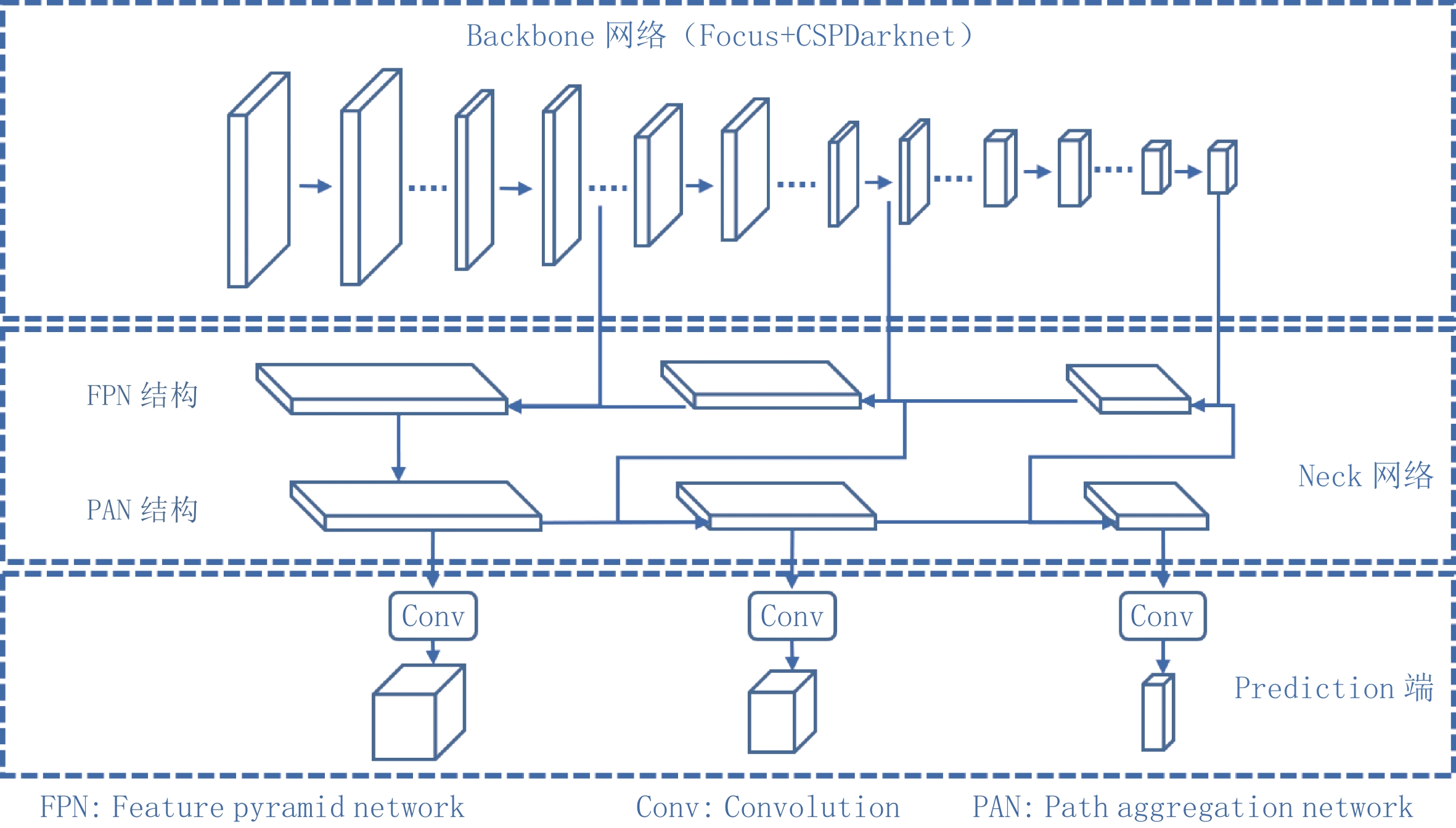
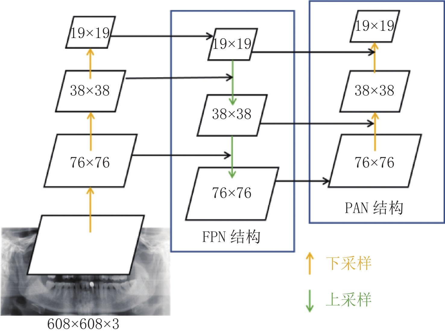
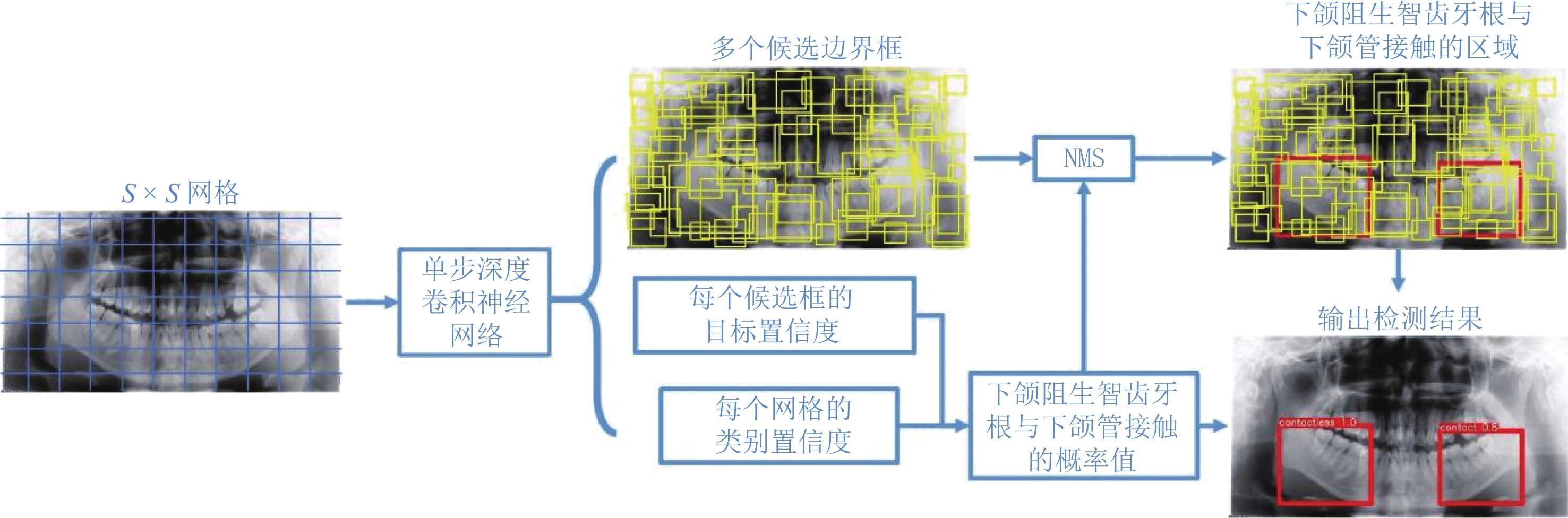
摘要: 为了提高曲面体层片中下颌阻生智齿牙根与下颌管位置关系的识别精度和效率,提出一种基于深度卷积神经网络的自动检测方法。该方法将下颌阻生智齿牙根与下颌管位置关系的自动检测视为回归任务与分类任务的结合,以YOLOv5网络为框架构建可同时完成分类和定位任务的深度卷积神经网络,将对应锥形束CT图像中获取的空间位置关系信息作为分类金标准,训练其学习曲面体层片图像特征与接触下颌管的智齿牙根之间的非线性关系。将新获得的曲面体层片输入到训练好的网络模型后,即可获得该曲面体层片下颌阻生智齿牙根与下颌管相互接触的概率值,同时预测出存在牙根与下颌管相互接触情况的区域。实验结果表明,本文方法能准确地判断出下颌阻生智齿牙根与下颌管是否接触,并能预测出存在牙根与下颌管相互接触情况的区域;与人工判读和其他方法相比,能获得更准确的检测结果。Abstract: To improve the accuracy and efficiency of identifying the relationship between the root of the impacted mandibular third molar (M3M) and the mandibular canal in panoramic radiographs, we proposed an automatic method based on a deep convolutional neural network. This method treats the automatic identification of the relationship between the root of the M3M and the mandibular canal as a combination of regression and classification tasks. It uses the YOLOv5 (You Only Look Once) network as a framework for constructing a deep convolutional neural network that can accomplish detection and classification tasks simultaneously. This network, which takes the spatial relationship information extracted from the corresponding cone-beam CT images as the ground-truth, was trained to learn the nonlinear relationship between image features and the root of the M3M contacting the mandibular canal. When inputting a newly acquired panoramic radiograph into the trained network, the network will output the probability value for the root of the M3M contacting the mandibular canal. In the meantime, the region that includes the root of the M3M contacting the mandibular canal can be predicted. The experimental results show that the proposed method can provide an accurate judgment of whether the roots of impacted mandibular wisdom teeth in the panoramic radiographs are in contact with the mandibular canal and the location of regions in which the roots of the M3M are in contact with the mandibular canals; compared to manual diagnosis and the other methods, the proposed method can obtain more accurate results.
-
随着年龄的增长,腰椎退行性变及椎间盘病变日趋增多,CT检查能及时发现诊断腰椎病变并能随访治疗效果,但CT检查辐射问题一直为人们所关注,随着患者受辐射剂量的增加,癌症的发生概率会增大,腰椎CT扫描范围包括性腺,而人体性腺对辐射最敏感,所以开展低剂量腰椎CT检查非常必要。
以往研究均是通过降低管电压或者降低管电流来降低辐射剂量,因腰椎体层较厚,降低管电压或管电流会导致图像噪声增加。本文为解决腰椎CT高辐射剂量及图像噪声偏高的问题,采用最新的能谱纯化技术结合高级模拟迭代重建(ADMIRE)技术,探讨如何更好的优化腰椎CT检查的图像质量和降低辐射剂量。
1. 材料与方法
1.1 一般资料
选取2021年8月至2022年5月因腰痛来我院行腰椎CT检查的患者,在检查前计算患者的体质量指数(bodymassindex,BMI),BMI=体重(kg)/身高(m)2。纳入年龄在25~65岁,BMI在18.5~25 kg/m2的患者,排除有腰椎手术史和腰椎畸形及有椎体金属植入物的患者,共收集88例。对照组(A组)、试验组(B组)每组44例。
A组与B组平均年龄分别为(45.9±12.1)岁和(47.2±13.8)岁。两组间年龄差异无统计学意义,A组与B组平均BMI分别为(20.1±2.89)kg/m2和(21.40±3.50)kg/m2。
1.2 扫描方法
采用德国SOMATOM Force第3代双源CT,扫描范围从胸12椎体至骶1椎体。扫描参数:对照组(A组)管电压120 kV,参考管电流350 mAs;试验组(B组)管电压Sn 150 kV,参考管电流350 mAs,其他扫描参数均一致。
重建采用高级模拟迭代重建算法(ADMIRE),重建等级3级,重建薄层图像,层厚1 mm,层间距0.60 mm,软组织窗采用软组织算法,卷积核Br40,骨窗采用骨算法,卷积核Br64,重建图像窗宽,窗位分别为350 HU和50 HU(软组织窗)、2500 HU和800 HU(骨窗)。所有图像重建完成后自动发至西门子Syngovia VB20A后处理工作站。
1.3 图像质量评价
1.3.1 客观评价
由1名主管技师从工作站中取L3椎体正中层面,在软组织窗上测量腰大肌与竖脊肌的CT值和噪声,腰大肌的噪声为SD1,竖脊肌的噪声为SD2,噪声值用对应所测的标准差表示,并计算信噪比(SNR):
$$ {\rm{SNR}}=腰大肌\;{\rm{CT}}\;值/{\rm{SD}}1。$$ (1) 1.3.2 主观评价
由3名副主任及以上诊断医师双盲法进行评分。评价L3/4层面椎间盘、椎间孔、黄韧带、硬膜囊及小关节图像质量。评价标准[1]:2分(软组织结构清晰,其边缘清楚,无伪影,且诊断明确);1分(软组织结构清晰,边缘欠清,有轻度伪影,但尚可诊断);0分(软组织结构不清,边缘模糊,伪影较重,不能进行诊断)。
1.4 辐射剂量
统计设备记录的容积CT剂量指数(CT dose index volumes,CTDIvol)及剂量长度乘积(dose length product,DLP),并计算有效辐射剂量(effective dose,ED)[2],计算公式:
$$ {\rm{ED}}={\rm{DLP}}\times k(k=0.011\;{\rm{mSv}}\cdot{\rm{mGy}}\cdot{\rm{cm}})。$$ (2) 1.5 统计学分析
1.5.1 客观评价和辐射剂量统计分析
采用SPSS 26.0软件对数据进行统计学分析。连续性数据非正态分布数据两组间比较采用Mann-Whitney U检验,用中位数及四分位数(M(Q25,Q75))表示。双侧检验,以P<0.05为差异有统计学意义。
1.5.2 主观评价
采用组内相关系数(intraclass correlation coefficient,ICC)对3位诊断医师的评分结果一致性进行分析。ICC介于0和1之间,ICC大于0.75表示一致性较好。
2. 结果
2.1 客观评价结果
两组图像腰大肌的CT值、竖脊肌的CT值和噪声(SD2)、SNR均存在统计学差异,而腰大肌的噪声(SD1)不具有统计学差异(表1);图1为120 kV轴位上噪声和CT值测量及矢状位重组图,图2为Sn 150 kV下的轴位上噪声和CT值测量测量及矢状位重组图。
表 1 A组和B组图像质量客观评价表Table 1. Objective evaluation of image quality in groups A and B项目 组别 统计检验 A组 B组 Z P 腰大肌/HU 53.00(48.70~56.00) 47.90(43.70~51.00) 2.741 0.016 SD1 5.73(4.83~6.83) 5.09(4.69~5.24) 1.904 0.057 竖脊肌/HU 52.00(46.2~55.00) 43.50(38.20~51) 3.511 <0.001 SD2 5.41(5.27~5.98) 4.56(3.62~5.63) 3.964 <0.001 SNR 9.12(7.88~10.51) 9.86(7.95~10.02) -0.693 0.488 ![]() 图 1 管电压120 kV下CT值和噪声测量及矢状位重组图(重组层厚1 mm、间隔0.6 mm)Figure 1. CT value, noise measurement, and sagittal position recombination at 120 kV tube voltage (recombination layer thickness 1 mm, interval 0.6 mm)
图 1 管电压120 kV下CT值和噪声测量及矢状位重组图(重组层厚1 mm、间隔0.6 mm)Figure 1. CT value, noise measurement, and sagittal position recombination at 120 kV tube voltage (recombination layer thickness 1 mm, interval 0.6 mm)![]() 图 2 管电压Sn 150 kV下CT值和噪声测量及矢状位重组图(重组层厚1 mm、间隔0.6 mm)Figure 2. CT value, noise measurement, and sagittal position recombination at tube voltage Sn 150 kV (recombination layer thickness 1 mm, interval 0.6 mm)
图 2 管电压Sn 150 kV下CT值和噪声测量及矢状位重组图(重组层厚1 mm、间隔0.6 mm)Figure 2. CT value, noise measurement, and sagittal position recombination at tube voltage Sn 150 kV (recombination layer thickness 1 mm, interval 0.6 mm)2.2 主观评价
3位医师对椎间盘、椎间孔、黄韧带、硬膜囊及小关节及整体图像质量评价均无统计学差异(表2),说明两组图像质量医师主观评价无差异,且均能符合医师诊断要求。
表 2 3位诊断医师的主观评分统计分析表Table 2. Statistical analysis of the subjective scores from the three doctors interpreting the computed tomography images指标 组别 P A组 B组 椎间盘 2.00±0.00 2.00±0.00 >0.999 椎间孔 1.98±0.15 1.98±0.15 0.156 黄韧带 1.95±0.21 2.00±0.00 0.562 硬膜囊 1.98±0.15 1.95±0.21 >0.999 小关节图像 2.00±0.00 2.00±0.00 0.320 整体图像质量 2.00±0.00 2.00±0.00 >0.999 2.3 辐射剂量
两组辐射剂量DLP、ED有统计学差异,两组辐射剂量差异明显,B组DLP值比A组降低了32.27%,B组ED值比A组降低了30.31%(表3)。
表 3 A组和B组辐射剂量统计表Table 3. Radiation dose in groups A and B项目 组别 统计检验 A组 B组 Z P mAs 333.00(300.00~362.00) 237.50(222.00~261.00) 7.885 <0.001 CTDIvol 14.75(13.65~16.00) 6.57(5.20~7.23) 8.015 <0.001 DLP 413.60(351.00~425.50) 280.13(230.89~327.20) 6.946 <0.001 ED 4.55(3.86~4.68) 3.08(2.54~3.60) 6.946 <0.001 3. 讨论
腰椎因体层相对较厚,需要高管电压来增加X线的穿透力,高管电流来降低图像的噪声,造成腰椎CT辐射剂量往往较高,以往研究都是通过降低管电流来降低辐射剂量。随着设备和技术的进步,众多新的降低辐射剂量的技术出现,如:低管电压[3-4]、自动管电流[5-6]、高级迭代重建算法[7]、能谱纯化[8]等,这些技术为我们开展低剂量CT提供了条件。
本研究B组管电压是用能谱纯化Sn 150 kV,而A组管电压是用120 kV,统计结果显示B组的辐射剂量低于A组30.31%。因为A组120 kV的X线球管是用铜和铝滤过,Sn 150 kV的X线球管是用能谱纯化技术的锡滤过,锡的原子序数比铜和铝高,锡滤过板能过滤掉X线球管的低能级射线,提高射线能量,而对人体产生辐射的主要是低能级软射线,低能级软射线以光电效应为主,大部分被人体吸收产生辐射。能谱纯化技术只保留了对人体成像有用的高能级射线,高能级射线会穿过人体相对辐射较少,所以B组辐射剂量低于A组,多学者也证实了这一说法[9-13]。
客观评价中A组肌肉的噪声要高于B组,腰大肌的噪声两组之间无统计学差异,而竖脊肌的噪声两组之间有统计学差异,此结果说明射线能量和图像噪声成正相关,也证实了Sn 150 kV的穿透力较120 kV的好。因竖脊肌处于腰大肌的下层,射线先穿过腰大肌再到竖脊肌,射线能量会因组织的阻挡发生衰减,A组射线的能量到达竖脊肌时比B组衰减更多,因衰减后的能量差异造成了噪声值的差异,故造成了两组不同肌肉之间统计学结果的差异。
沈梓璇等[14]论述了120 kVp管电压所获得的腰椎图像质量评分以及信噪比皆较高,但辐射剂量也较大的观点。本文为了解决这一问题,首次采用Sn 150 kV用于腰椎CT检查,主观评价结果显示,3位观察者的ICC为0.829,表示为两组图像主观评价一致性较好,说明两组图像质量均满足诊断要求,主客观评价结果均证实了Sn 150 kV用于腰椎CT检查是可行的。王帅等[15]也证实Sn 150 kV能用于全腹部CT检查,且辐射剂量较低,与本文研究结果一致。
高级模拟迭代重建,是将原始图像中的原始数据噪声投射到图像中,得到的图像是多次迭代重建后的组合,再将原始数据进行准确的图像校正,对原始数据域进行去噪及去除伪影,最后进行图像域的校正,反复迭代来降低噪声,图像空间分辨率不受影响。客观评价表中A组和B组图像的噪声均值都处于10以下,证实了高级模拟迭代重建的降噪能力。顾海峰等[16]和Schlunk等[17]也证明了迭代重建能降低噪声保证图像质量满足诊断需求。
综上所述,采用能谱纯化Sn 150 kV结合ADMIRE,不但能有效减低辐射剂量,还可保证优质的图像质量,值得在成人腰椎CT中推广使用。
-
![]()
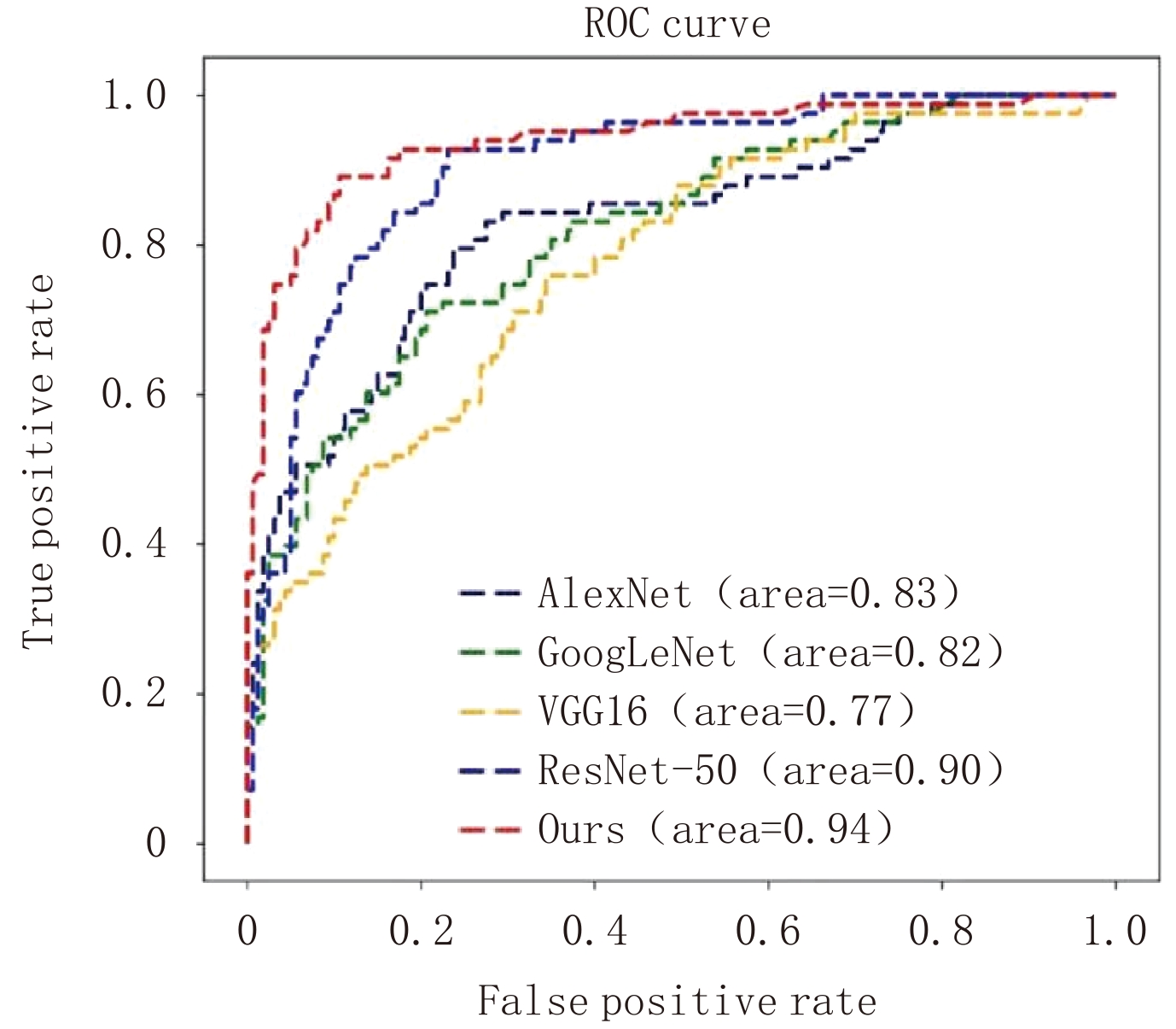
图 4 使用不同模型获得结果对应ROC曲线的对比
Figure 4. The comparison of corresponding ROC curves of the results obtained using the different models
![]()
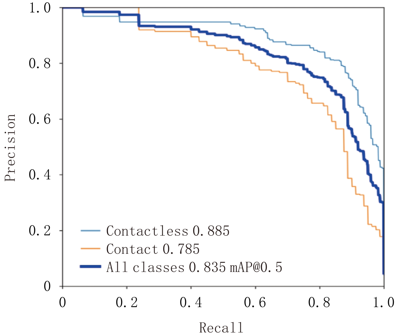
图 5 使用本文方法所得结果对应的PR曲线
Figure 5. The PR curves corresponding to the results obtained using the method in this paper
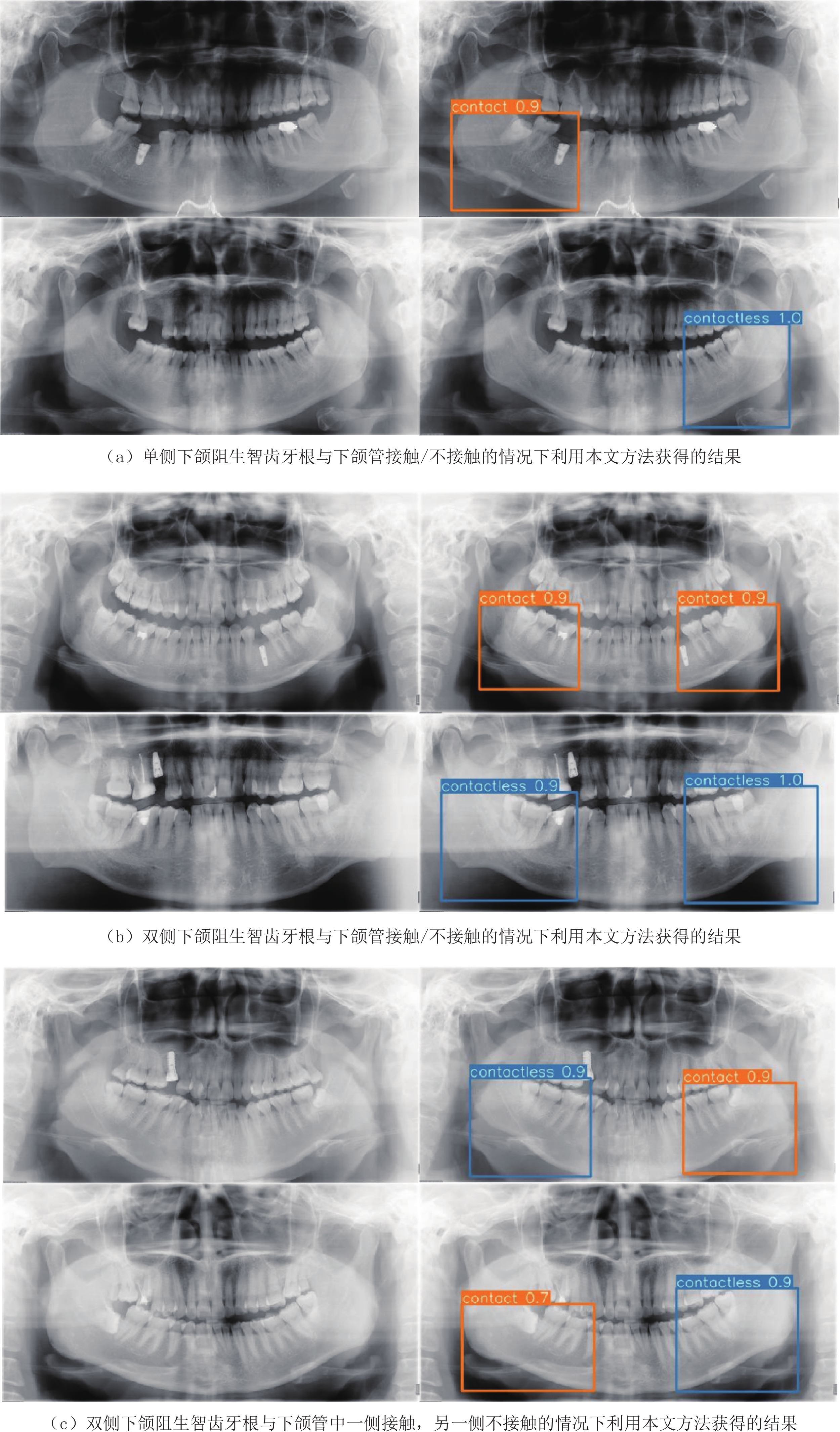
![]()
图 6 使用本文方法得到的输出结果
每一行左侧图像均为原始图像,右侧是本文方法输出结果图。结果图中的棕色字符contact代表下颌阻生智齿牙根与下颌管的位置关系是接触状态,蓝色字符contactless代表两者没有接触;棕色数字是预测为接触的置信度,蓝色数字是预测为不接触的置信度。
Figure 6. Demonstration of the output results obtained from the proposed method in this paper
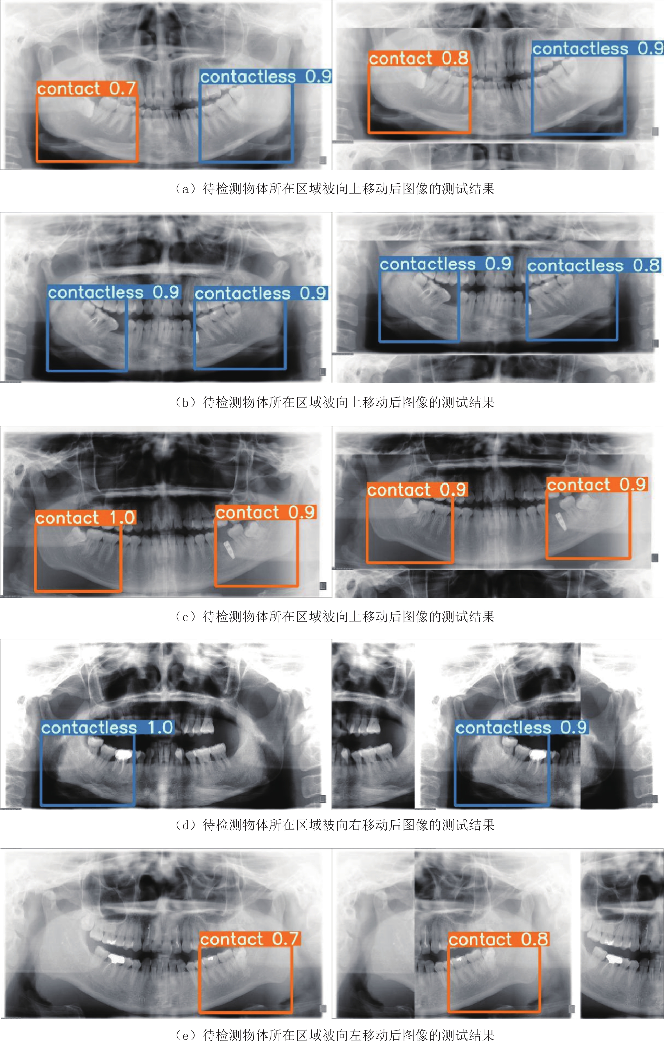
![]()
图 7 待检测物体所在区域被不同方向移动后图像的部分测试结果
Figure 7. Some examples of predicted results, after the regions including the objects to be detected in panoramic images, have been shifted in different directions
表 1 Backbone网络涉及的主要参数
Table 1 The main parameters of the backbone network
模块名称 数量 卷积核 尺寸 步长 输入尺寸 输出尺寸 Conv 1 80 3⊆3 2 608⊆608⊆3 304⊆304⊆80 Conv 1 160 3⊆3 2 304⊆304⊆80 152⊆152⊆160 CSP1_4 4 160 - - 152⊆152⊆160 152⊆152⊆160 Conv 1 320 3⊆3 2 152⊆152⊆160 76⊆76⊆320 CSP1_8 8 320 - - 76⊆76⊆320 76⊆76⊆320 Conv 1 640 3⊆3 2 76⊆76⊆320 38⊆38⊆640 CSP1_12 12 640 - - 38⊆38⊆640 38⊆38⊆640 Conv 1 1280 3⊆3 2 38⊆38⊆640 19⊆19⊆1280 CSP1_4 4 1280 - - 19⊆19⊆1280 19⊆19⊆1280 SPPF 1 1280 - - 19⊆19⊆1280 19⊆19⊆1280  下载: 导出CSV
表 2 本文方法与其他方法及人工判读所得预测结果对应的分类性能评价指标的对比
Table 2 The comparison of classification performance for the proposed method, manual diagnosis, and the other models
方法 准确率 灵敏度 特异度 精确度 人工判读 0.845 0.741 0.892 0.759 AlexNet 0.778 0.506 0.919 0.764 GoogLeNet 0.770 0.434 0.944 0.800 VGG-16 0.737 0.422 0.900 0.686 ResNet-50 0.831 0.663 0.919 0.809 本文方法 0.881 0.819 0.913 0.829
下载: 导出CSV
表 3 部分概率阈值对应的分类性能评价指标值
Table 3 The measurements of classification performance for different thresholds
概率阈值 准确率 灵敏度 特异度 精确度 0.60 0.881 0.819 0.913 0.829 0.65 0.881 0.795 0.925 0.846 0.70 0.868 0.747 0.931 0.849 0.75 0.860 0.699 0.944 0.866
下载: 导出CSV
表 4 使用本文方法时,不同训练迭代次数、批大小、学习率以及优化器参数对应的各分类性能指标值
Table 4 The measurements of classification performance for different iterations, epochs, learning rates, and parameters of the optimizer in the proposed method
参数名称 参数取值 准确率 灵敏度 特异度 精确度 训练迭代次数 800 0.877 0.807 0.913 0.827 1200 0.881 0.819 0.913 0.829 1600 0.835 0.614 0.95 0.864 批大小 4 0.840 0.602 0.963 0.893 6 0.881 0.819 0.913 0.829 学习率 0.0022 0.889 0.759 0.956 0.900 0.0032 0.881 0.819 0.913 0.829 0.0042 0.823 0.590 0.944 0.845 优化器参数β1(β2=0.999) 0.743 0.868 0.723 0.944 0.870 0.843 0.881 0.819 0.913 0.829 0.943 0.864 0.747 0.925 0.838 优化器参数β2(β1=0.843) 0.9 0.856 0.675 0.950 0.875 0.99 0.868 0.759 0.925 0.840 0.999 0.881 0.819 0.913 0.829
下载: 导出CSV
表 5 本文所用深度网络与其他模型涉及参数数量的对比
Table 5 The comparison of the number of parameters used in our network and the others
网络模型 AlexNet GoogLeNet VGG-16 ResNet-50 本文方法 参数量/M 61.0 7.0 138.4 25.5 87.3
下载: 导出CSV
表 6 待检测物体所在区域朝不同方向移动前和移动后,本文方法对测试图像所得预测结果的分类性能评价指标对比
Table 6 The comparison of classification performance for the predicted results between the cases with or without the regions including the targets shifted in different directions
方法 准确度 灵敏度 特异度 精确度 移动前 0.881 0.819 0.913 0.829 移动后 0.864 0.723 0.938 0.857
下载: 导出CSV
-
[1] 王东苗, 金致纯, 丁旭, 等. 锥形束CT评估下颌阻生智齿拔除术后下牙槽神经损伤的风险[J]. 南京医科大学学报(自然科学版), 2016,36(10): 1263−1266. [2] WANG D M, HE X T, WANG Y L, et al. Topographic relationship between root apex of mesially and horizontally impacted mandibular third molar and lingual plate: Cross-sectional analysis using CBCT[J]. Scientific Reports, 2016, 6(1): 39268−39278. doi: 10.1038/srep39268
[3] EKERT T, KROIS J, MEINHOLD L, et al. Deep learning for the radiographic detection of apical lesions[J]. Journal of Endodontics, 2019, 45(7): 917−922. doi: 10.1016/j.joen.2019.03.016
[4] CHANG H J, LEE S J, YONG T H, et al. Deep learning hybrid method to automatically diagnose periodontal bone loss and stage periodontitis[J]. Scientific Reports, 2020, 10(1): 7531−7539. doi: 10.1038/s41598-020-64509-z
[5] ARIJI Y, YANASHITA Y, KUTSUNA S, et al. Automatic detection and classification of radiolucent lesions in the mandible on panoramic radiographs using a deep learning object detection technique[J]. Oral Surgery, Oral Medicine, Oral Pathology and Oral Radiology, 2019, 128(4): 424−430. doi: 10.1016/j.oooo.2019.05.014
[6] VINAYAHALINGAM S, TONG X, BERGÉ S, et al. Automated detection of third molars and mandibular nerve by deep learning[J]. Scientific Reports, 2019, 9(1): 9007−9014. doi: 10.1038/s41598-019-45487-3
[7] LEE J, KIM D, JEONG S. Diagnosis of cystic lesions using panoramic and cone beam computed tomographic images based on deep learning neural network[J]. Oral Diseases, 2020, 26(1): 152−158. doi: 10.1111/odi.13223
[8] FUKUDA M, ARIJI Y, KISE Y, et al. Comparison of 3 deep learning neural networks for classifying the relationship between the mandibular third molar and the mandibular canal on panoramic radiographs[J]. Oral Surgery, Oral Medicine, Oral Pathology and Oral Radiology, 2020, 130(3): 336−343. doi: 10.1016/j.oooo.2020.04.005
[9] CHOI E, LEE S, JEONG E, et al. Artificial intelligence in positioning between mandibular third molar and inferior alveolar nerve on panoramic radiography[J]. Scientific Reports, 2022, 12(1): 2456−2463. doi: 10.1038/s41598-022-06483-2
[10] ZWA B, LJA B, SHUAI W. Apple stem/calyx real-time recognition using YOLO-v5 algorithm for fruit automatic loading system[J]. Postharvest Biology and Technology, 2022, 185(2): 111808−111815.
[11] BOCHKOVSKIY A, WANG C Y, LIAO H. YOLOv4: Optimal speed and accuracy of object detection[J]. arXiv Preprint, 2020, arXiv: 2004.10934v1.
[12] LIN T Y, DOLLAR P, GIRSHICK R, et al. Feature pyramid networks for object detection[C]//IEEE Conference on Computer Vision and Pattern Recognition (CVPR). 2017: 2117-2125.
[13] LI H, XIONG P, AN J, et al. Pyramid attention network for semantic segmentation[J]. arXiv Preprint, 2018, arXiv:1805.10180.
[14] REZATOFIGHI H, TSOI N, GWAK J Y. Generalized Intersection over Union: A metric and a loss for bounding box regression[C]//IEEE Conference on Computer Vision and Pattern Recognition (CVPR). 2019: 658-666.
[15] COOK N R. Use and misuse of the receiver operating characteristic curve in risk prediction[J]. Circulation, 2007, 115(7): 928−35. doi: 10.1161/CIRCULATIONAHA.106.672402
[16] BUCKLAND M K, GEY F C. The relationship between recall and precision[J]. Journal of the Association for Information Science & Technology, 2010, 45(1): 12−19.
-
期刊类型引用(2)
1. 涂立冬,李雅萍. 岩土勘查技术在盐矿绿色矿山建设中的应用初探. 盐科学与化工. 2025(04): 9-12 .  百度学术
百度学术
2. 杨兆林,潘懿,白旭晨,刘禄平. 露天铁矿采空区隐蔽致灾普查与防治措施应用研究. 矿业研究与开发. 2024(09): 74-81 . 百度学术
其他类型引用(2)


计量
- 文章访问数: 398
- HTML全文浏览量: 136
- PDF下载量: 43
- 被引次数: 4
