
Application Value of Personalized Contrast Agent Injection Schemes of Different Durations in Pulmonary Artery CTA
-
摘要:
目的:研究不同时长的个性化对比剂注射方案在提升肺动脉CTA的图像质量和降低对比剂潜在风险的应用价值。资料与方法:2023年1月至2024年10月临床怀疑为肺动脉栓塞的患者106例作为研究对象,随机将患者分配到A、B两组。采用独立样本t检验,比较两组间的上腔静脉的CT值、肺动脉主干的CT值、左肺动脉及右肺动脉的CT值、左房的CT值;两组间的图像质量主观的综合评分;以P < 0.05为具有统计学意义。结果:两组间对比剂注射总量、注射时长和注射速率进行比较,B组对比剂的注射总量和注射时长都低于A组,其差异有统计学意义。两组间的右肺动脉、左肺动脉、左房CT值比较接近,无统计学差异,两组间的上腔静脉CT值差异有统计学差异;两组间的图像质量主观评分比较,有统计学差异,B组>A组。结论:采用8s时长的个性化对比剂注射方案不仅可以提高肺动脉CTA的总体图像质量,还可以有效减少对比剂用量,同时缩短注射时长。
Abstract:Objective: This study investigated the application value of personalized contrast agent injection schemes of different durations in improving the image quality of pulmonary artery CTA and reducing the potential risk associated with contrast agents. Materials and Methods: From January 2023 to October 2024, 106 patients with suspected pulmonary embolism were randomly assigned to Groups A and B. Using the independent samples t-test, we compared the CTA values of the superior venae cavae, pulmonary artery trunks, left and right pulmonary arteries, and left atria of the two groups. We also compared the subjective comprehensive evaluations of the CTA image quality of the two groups; a value of P<0.05 was considered statistically significant. Additionally, the two groups were compared in terms of the total amount of contrast agent injection, injection duration, and injection rate. Both the total amount and duration of contrast agent injection in Group B were lower than those in Group A; the concomitant difference was statistically significant. The CTA values of the right and left pulmonary arteries and the left atria of the two groups were relatively close, with no statistically significant difference. However, a statistically significant difference in the CTA values of the superior venae cavae of the two groups was observed. The subjective evaluation of image quality between the two groups indicated a statistically significant difference (P=0.04), with the image quality of Group B being higher than that of Group A. Conclusion: The use of an 8s personalized contrast agent injection regimen can not only improve the overall image quality of pulmonary artery CTA but also reduce the amount of contrast agent used and shorten the injection duration.
-
随着地震勘探难度的提升,仅依据地震振幅信息难以实现高精度的地震勘探需求,故结合岩石物理信息,利用频散属性和介质的粘弹性等对储层特征进行刻画成为现今研究热点[1]。目前常见的含油气储层大多为裂隙多孔介质,研究发现,当地震波在裂隙多孔介质中传播时,由于受到波致流(宏观Biot流、介观层间流和微观喷射流)的影响,地震波会发生明显的衰减和频散[2-5],具有粘弹介质传播特性。然而,常规流体检测方法一般基于Biot孔隙弹性理论,没有考虑地震波粘弹介质传播特性,降低了流体识别精度。因此,基于粘弹介质地震岩石物理模型,构建能够更加准确描述流体性质的流体因子,开发相应的地震反演技术,对流体预测描述具有重要意义。
储层流体识别是一项基于流体因子对流体的敏感性进行流体判别的重要技术。因此,构建对流体更为敏感的流体因子是储层流体精准识别的技术关键。流体因子的概念最早是Smith等[6]提出的,特指由纵、横波速度相对变化量的而运算构成的参数。随后,Biot[7]和Gassmann[8]分析了多孔流体饱和岩石的弹性参数构建方法;Russell等[9]利用Biot-Gassmann方程,推导了Gassmann流体项作为流体指示因子;Zong等[10]消除了岩石骨架的影响,构建并反演了固液解耦流体因子作为流体识别指标,然而其缺乏对孔裂隙喷射流引起的衰减的考虑。
由于裂隙的存在会导致岩石在外力作用下产生挤喷流现象,并导致介质呈现粘滞性特征[11-12]。为了更好地描述该现象,Tang等[13-14]分别考虑了硬币型裂隙和钹状裂隙模型中喷流效应的影响,构建了描述孔隙、裂隙并存时的弹性波统一理论,该理论能够更加准确描述弹性波在介质中的传播特征,以此提高流体识别的精度。
地震频变反演是基于粘弹介质理论形成的预测流体的常用方法,而常用的频变反演方法主要有两种,一种是频变AVO反演方法[15-17],另一种是基于弹性阻抗的频变反演方法[18-20]。频变AVO反演利用的是反射系数近似公式,而基于弹性阻抗的频变反演是通过构建弹性阻抗与弹性参数的弹性阻抗方程,利用弹性阻抗方程进行反演。在弹性阻抗反演方法中,假设弹性阻抗的对数的梯度和反射系数成正比,建立弹性阻抗与反射系数之间的关系,从而将反射系数方程改写为弹性阻抗方程[18,21-22]。
Connolly[23]通过对叠后波阻抗和AVO特点的分析,提出了一种同时考虑波阻抗和AVO特征的弹性阻抗反演方法。Yin等[21]基于Russell提出的多空流体饱和弹性阻抗近似方程,提出了包含Gassmann流体项的弹性阻抗方程,并通过弹性阻抗反演实现流体项反演的方法。Zong等[18]提出了粘弹性介质的弹性阻抗方程,并考虑参数的频变特征,实现粘弹性介质Russell流体因子的频变反演。频变弹性阻抗反演相比于频变AVO反演表现出更强的优势[22],因此,为了更好的提取与频率相关的新流体因子,本研究开发基于弹性阻抗反演的方法。
在前人的研究基础上,本研究综合利用岩石物理分析,构建粘弹频变固液解耦流体因子,该因子能够保持原有流体因子的基本特征,并且能够提高含对孔隙、裂隙介质中流体的预测能力。同时,探讨基于弹性阻抗的叠前地震频变反演方法,及其在胜利油田胜北地区复杂砂岩储层流体检测中的应用。模型试算和实际资料处理结果表明,基于粘弹频变固液解耦流体因子叠前地震反演的储层含油气性预测方法,能够提取孔裂隙频变粘弹固液解耦流体因子。预测结果能够有效区分储层的流体类型,准确刻画储层流体边界,消除流体识别假象,提高流体识别精度。
1. 基于频变反演的流体识别方法原理
1.1 频变敏感参数构建与分析
地震勘探方法自提出以来,经历了构造解释、储层描述和流体识别3个发展阶段,其中流体识别技术作为勘探开发的前沿技术,需要作为长期研究的课题。而在流体识别方法方面,采用流体指示因子来进行流体判别受到了广泛关注。相比于常规流体因子,频变流体因子由于充分考虑了频率对岩石弹性参数的影响,展示了其在区分烃类流体方面的独特能力[24]。因此,有必要构建敏感程度更高的频变敏感参数。首先,根据Biot-Gassman[8,25]理论,在低频条件下的饱和流体体积模量可以写为:
$$ {K_{{\mathrm{sat}}}} = {K_{\mathrm{d}}} + {\kappa ^2}\chi \text{,} $$ (1) 其中:
$\kappa = 1 - {{{K_{\mathrm{d}}}} / {{K_{\mathrm{s}}}}}$ ,表示Biot系数;$ 1/\chi=(\kappa-\phi)/K_{\mathrm{s}}+\phi/K\mathrm{_f}\mathrm{ } $ ,$ {K_{{\mathrm{sat}}}} $ 、$ {K_{\mathrm{d}}} $ 和$ {K_{\mathrm{s}}} $ 分别为饱和岩石体积模量、干岩石体积模量和岩石基质体积模量;$ {K_{\mathrm{f}}} $ 为饱和流体体积模量,$ \phi $ 为岩石有效孔隙度。考虑到孔裂隙挤喷流体流动,Tang[13]在2011年提出了考虑硬币型裂隙挤喷流效应的饱和岩石体积模量。由于硬币型模型中孔隙与裂隙的流体交换处于硬币的边缘,然而,在力学理论方面,裂隙在硬币边缘处是处于闭合状态的。因此,为了进一步改进模型,Tang等[14]在2012年又提出了钹状裂隙模型,将流体交换位置改变到了硬币模型的中部。该种模型的饱和岩石体积模量可以统一表示为:
$$ {K_{{\mathrm{sat}}}} = {K_{\mathrm{d}}} + \frac{{{\kappa ^2}\chi }}{{1 + S\left( \omega \right)\chi }} \text{,} $$ (2) 其中:
$ S\left( \omega \right) $ 为描述孔裂隙相互作用的挤喷流函数。在本研究中,为了充分考虑孔裂隙挤喷流效应对流体识别的影响,消除流体识别的误差,同时将两种模型耦合到一起,因此,
$ S\left( \omega \right) $ 可以表示为:$$ S(\omega ) = {S_1}(\omega ) + {S_2}(\omega ) \text{,} $$ (3) $$ {S_1}\left( \omega \right) = \frac{8}{3}\text{π} \varepsilon \frac{{\left( {1 - \nu } \right)}}{\mu }f\left( \zeta \right)\frac{\left( {\displaystyle \frac{{{1/ {{K_{\mathrm{d}}} - }}{1 / {{K_{\mathrm{s}}}}}}}{{{1/ {{K_{\mathrm{d}}} - }}{1/ {{K_0}}}}} - f\left( \zeta \right)} \right)}{\left( {1 + \displaystyle \frac{{4\left( {1 - v} \right){K_{\mathrm{f}}}}}{{3\mu \gamma }}\Big( {1 - f\left( \zeta \right)} \Big)} \right)} \text{,} $$ (4) $$ {S_2}\left( \omega \right){\text{ = }}\frac{{8\varepsilon \left( {1 - \nu } \right){{\left( {1 + \lambda } \right)}^3}}}{{3\mu }} \times \frac{{\left( {\displaystyle\dfrac{{{1 / {{K_0}}} - {1 / {{K_{\mathrm{s}}}}}}}{{{1 / {{K_{\mathrm{d}}}}} - {1 / {{K_0}}}}}} \right)M}}{{1 - \displaystyle\dfrac{{3i\omega \eta \left( {1 + 2\lambda } \right)}}{{2{K_{\mathrm{f}}}\lambda {\gamma ^2}}}\left( {1 + \displaystyle\dfrac{{4\left( {1 - \nu } \right){K_{\mathrm{f}}}{{\left( {1 + \lambda } \right)}^3}}}{{3\text{π} \mu \gamma \left( {1 + 2\lambda } \right)}}M} \right)}} \text{,} $$ (5) $$ f\left(\zeta \right)=\frac{2{J}_{1}\left(\zeta \right)}{\zeta {J}_{0}\left(\zeta \right)}\text{,}\zeta =\left({\frac{3i\omega \eta }{{\gamma }^{2}{K}_{{\mathrm{f}}}}} \right)^{\tfrac{1}{2}}\text{,} $$ (6) 其中:
$ {S_1}(\omega ) $ 和$ {S_2}(\omega ) $ 分别为硬币型和钹状裂隙挤喷流函数;$ \lambda = {\left( {\displaystyle\frac{{3\phi }}{{4\text{π} \varepsilon }}} \right)^{\tfrac{1 }{ 3}}} $ ,$ M = 1 + \displaystyle\frac{{4 - 5\nu }}{{2(7 - 5\nu )}}\frac{{{\lambda ^3}}}{{{{(1 + \lambda )}^3}}} + \displaystyle\frac{9}{{2(7 - 5\nu )}}\frac{{{\lambda ^5}}}{{{{(1 + \lambda )}^5}}} $ ,$\omega $ 为圆周角频率,$\lambda $ 为孔裂隙尺度比,$\varepsilon $ 、$\eta $ 和$\gamma $ 分别表示裂隙密度、孔隙流体粘滞系数和裂隙纵横比,$ \nu $ 为干燥介质泊松比;当$S(\omega ) = 0$ 时,岩石体积模量为$ {K_0} $ ;$ {J_0}( * ) $ 和$ {J_1}( * ) $ 分别为第一类零阶和一阶贝塞尔函数;${K_{\mathrm{d}}}$ 和${K_{\mathrm{s}}}$ 分别为干岩石体积模量和岩石基质体积模量,${K_{\mathrm{f}}}$ 为饱和流体体积模量;$\mu $ 为剪切模量,$i$ 为虚数单位。通过将式(2)与Gassmann流体项
$f$ 进行关系构建可得,$$ {K_{{\mathrm{sat}}}} = {K_{\mathrm{d}}} + \frac{f}{{1 + S\left( \omega \right)\chi }} 。 $$ (7) 因此有,
$$ f = S \cdot {\kappa _\phi } \cdot {K_{\mathrm{{fs}}}} \text{,} $$ (8) 其中:
$$ {K_{{\mathrm{fs}}}} = \frac{{{K_{\mathrm{f}}}}}{S} \text{,} $$ (9) $$ S = 1 + S(\omega )\chi \text{,} $$ (10) $$ {\kappa _\phi } = \frac{{{\kappa ^2}}}{\phi } 。 $$ (11) 我们将
$ {K_{{\mathrm{fs}}}} $ 称为孔裂隙固液解耦流体因子,$ S $ 为耦合挤喷流效应项,$ {\kappa _\phi } $ 为与孔隙度相关的Biot系数项。为了流体判别精度的提高,将Futterman[26]近似常 Q模型引入粘弹介质,构建孔裂隙粘弹固液解耦流体因子为:
$$ \begin{aligned}K_{\mathrm{f}\mathrm{\mathit{s}}_{\mathrm{ane}}}=\kappa_{\phi}^{-1}S^{-1}f_{\mathrm{ane}}=\kappa_{\phi}^{-1}S^{-1}\left(\rho V_p^2-\gamma_{\mathrm{dry}}^2\rho V_s^2\right)+\quad\qquad \\ \kappa_{\phi}^{-1}S^{-1}\left(\begin{gathered}\rho V_p^2\left(\frac{2}{\text{π}Q_p}log\left(\frac{\omega}{\omega_{\mathrm{r}}}\right)-\frac{i}{Q_{\mathrm{p}}}\right) \\ -\gamma_{\mathrm{dry}}^2\rho V_s^2\left(\frac{2}{\text{π}Q_{\mathrm{s}}}log\left(\frac{\omega}{\omega_{\mathrm{r}}}\right)-\frac{i}{Q_{\mathrm{s}}}\right)\end{gathered}\right)=K_{\mathrm{f}s_{\mathrm{ela}}}+\Delta K_{\mathrm{f}s_{\mathrm{Q}}}\end{aligned}\text{,} $$ (12) 其中:
$ {Q_{\mathrm{p}}} $ 和$ {Q_{\mathrm{s}}} $ 分别为纵波和横波品质因子,$ \omega $ 和$ {\omega _{\mathrm{r}}} $ 分别为圆周角频率和参考频率,$i$ 为虚数单位。为了验证新提出的孔裂隙粘弹固液解耦流体因子的频率敏感性的优势,分别对纵波速度、横波速度、泊松比、体积模量、杨氏模量、剪切模量、固液解耦流体因子和孔裂隙粘弹固液解耦流体因子进行了分析,模型参数如表1所示,结果如图1所示。
表 1 弹性参数敏感性分析模型数据Table 1. Sensitivity analysis data of elastic parameters岩性 $ V_{\mathrm{P}} $/(m/s) $ V_{\mathrm{s}} $/(m/s) $ \mathrm{\rho} $/(g/cm3) $ {Q}_{{\mathrm{p}}1}$ $ {Q}_{{\mathrm{p}}2} $ $ {Q}_{{\mathrm{s}}} $ 砂岩 2590 1060 2.210 10 20 120 分析结果表明,孔裂隙粘弹固液解耦流体因子对纵波衰减和频率的敏感程度较高,可以作为流体指示因子用来流体检测。
为对比孔裂隙粘弹固液解耦流体因子与其他弹性参数的频散程度,本文优选流体因子,进一步分析不同弹性参数与孔裂隙粘弹固液解耦流体因子的频散程度,分析结果如图2所示。图2的计算过程使用表1中的模型参数。
![]() 图 2 不同弹性参数频散程度分析Figure 2. Analysis of dispersion degree of different elastic parameters
图 2 不同弹性参数频散程度分析Figure 2. Analysis of dispersion degree of different elastic parameters计算结果表明,相较于固液解耦流体因子、拉梅参数和体积模量等弹性参数,本文新提出的孔裂隙粘弹固液解耦流体因子的频散程度最高,并且比固液解耦流体因子的频散程度高15% 左右。因此,我们在胜北断层下降盘A井区储层含油气识别中,将孔裂隙粘弹固液解耦流体因子作为油气指示因子,提高储层流体识别的可靠性。
1.2 基于叠前地震反演的储层含油气性预测方法
借鉴Connolly[23]构建的反射系数与弹性阻抗的关系,Lan等[20]建立了频变弹性阻抗反射系数方程,并发展了基于弹性阻抗的频变反演算法。基于Biot-Gassmann理论,Russel等[9,27]对饱含流体孔隙介质模型进行了分析,推导得到了Gassmann流体项的反射系数近似公式为:
$$ R_{{\mathrm{pp}}}^{{\mathrm{ane}}}\left( \theta \right) =\Biggr( {\left( {1 - \frac{{\gamma _{{\mathrm{dry}}}^2}}{{\gamma _{{\mathrm{sat}}}^2}}} \right)\frac{{{{\sec }^2}\theta }}{4}} \Biggr)\frac{{\Delta {f_{{\mathrm{ane}}}}}}{{{f_{{\mathrm{ane}}}}}} + \left( {\frac{{\gamma _{{\mathrm{dry}}}^2}}{{4\gamma _{{\mathrm{sat}}}^2}}{{\sec }^2}\theta - \frac{2}{{\gamma _{{\mathrm{sat}}}^2}}{{\sin }^2}\theta } \right)\frac{{\Delta \mu }}{\mu } + \left( {\frac{1}{2} - \frac{{{{\sec }^2}\theta }}{4}} \right)\frac{{\Delta \rho }}{\rho } \text{,} $$ (13) 其中:
${\gamma _{{\mathrm{dry}}}}$ 和${\gamma _{{\mathrm{sat}}}}$ 分别为干岩石骨架纵横波速度比和饱和岩石纵横波速度比,$\rho $ 为岩石密度,$\mu $ 表示剪切模量,${f_{{\mathrm{ane}}}}$ 为Gassmann流体项。通过式(8)的关系,将式(13)变换为孔裂隙粘弹固液解耦流体因子的反射系数近似方程为:
$$ \begin{aligned}R_{\mathrm{pp}}^{\mathrm{ane}}\left(\theta\right)=\left(\frac{\sec^2\theta}{4}-\frac{\gamma_{\mathrm{dry}}^2}{4\gamma_{\mathrm{sat}}^2}\sec^2\theta\right)\frac{\Delta K_{fs_{\mathrm{ane}}}}{K_{fs_{\mathrm{ane}}}}+\left(\frac{\gamma_{\mathrm{dry}}^2}{4\gamma_{\mathrm{sat}}^2}\sec^2\theta-\frac{2}{\gamma_{\mathrm{sat}}^2}\sin^2\theta\right)\frac{\Delta\mu_s}{\mu_s}\quad \\ +\left(\frac{\sec^2\theta}{4}-\frac{2}{\gamma_{\mathrm{sat}}^2}\sin^2\theta\right)\frac{\Delta S}{S}+\left(\frac{\sec^2\theta}{4}-\frac{\gamma_{\mathrm{dry}}^2}{4\gamma_{\mathrm{sat}}^2}\sec^2\theta\right)\frac{\Delta\kappa_{\phi}}{\kappa_{\phi}}+\left(\frac{1}{2}-\frac{\sec^2\theta}{4}\right)\frac{\Delta\rho}{\rho}\end{aligned}\text{,} $$ (14) 其中:
${\mu _s} = {\mu \mathord{\left/ {\vphantom {\mu S}} \right. } S}$ 。考虑粘弹介质,并借鉴Connolly[23]构建的反射系数与弹性阻抗的关系,构建得到孔裂隙粘弹固液解耦流体因子弹性阻抗反射系数特征方程为:
$$ {{\Delta }}\ln \Big({{{\mathrm{EI}}}}_{{Q}}(\theta ,\omega )\Big) = a(\theta ,\omega )\frac{{\Delta {K_{f{s_{{\mathrm{ane}}}}}}}}{{{K_{f{s_{{\mathrm{ane}}}}}}}}(\omega ) + b(\theta ,\omega )\frac{{\Delta {\mu _s}}}{{{\mu _s}}}(\omega ) + c(\theta ,\omega )\frac{{\Delta S}}{S}(\omega ) + d(\theta )\frac{{\Delta {\kappa _\phi }}}{{{\kappa _\phi }}} + e(\theta )\frac{{\Delta \rho }}{\rho } \text{,} $$ (15) $$ \left\{\begin{gathered} a(\theta ,\omega ) = \frac{{{{\sec }^2}\theta }}{2} - \frac{{\gamma _{{\mathrm{dry}}}^2}}{{2\gamma _{{\mathrm{sat}}}^2}}\Biggr( {1 - \frac{2}{{\text{π} {Q_p}}}\log \left( {\frac{\omega }{{{\omega _r}}}} \right)} \Biggr){\sec ^2}\theta \\ b(\theta ,\omega ) = \left( {\frac{{\gamma _{{\mathrm{dry}}}^2}}{{2\gamma _{{\mathrm{sat}}}^2}}{{\sec }^2}\theta - \frac{4}{{\gamma _{{\mathrm{sat}}}^2}}{{\sin }^2}\theta } \right)\Biggr( {1 - \frac{2}{{\text{π} {Q_p}}}\log \left( {\frac{\omega }{{{\omega _r}}}} \right)} \Biggr) \\ c(\theta ,\omega ) = \frac{{{{\sec }^2}\theta }}{2} - \frac{4}{{\gamma _{{\mathrm{sat}}}^2}}\Biggr( {1 - \frac{2}{{\text{π} {Q_p}}}\log \left( {\frac{\omega }{{{\omega _r}}}} \right)} \Biggr){\sin ^2}\theta \\ d(\theta ) = \frac{{{{\sec }^2}\theta }}{2} - \frac{{\gamma _{{\mathrm{dry}}}^2}}{{2\gamma _{{\mathrm{sat}}}^2}}\Biggr( {1 - \frac{2}{{\text{π} {Q_p}}}\log \left( {\frac{\omega }{{{\omega _r}}}} \right)} \Biggr){\sec ^2}\theta \\ e(\theta ) = 1 - \frac{{{{\sec }^2}\theta }}{2} \\ \end{gathered} \right.\text{,} $$ (16) 其中
$ \mathrm{EI}_Q $ 为粘弹介质弹性阻抗。最后,式(15)中的弹性参数对频率求偏导,构建孔裂隙频变粘弹固液解耦流体因子
$ I_{K_{\mathrm{f}s_{\mathrm{ane}}}} $ 、孔裂隙频变剪切模量$ {I_{{\mu _s}}} $ 和频变挤喷流模量$ {I_S} $ ,如式(17)所示:$$ \begin{gathered} {I_{{K_{{\mathrm{f}}{s_{{\mathrm{ane}}}}}}}} = \exp \left( {\frac{{{{\partial {K_{f{s_{{\mathrm{ane}}}}}}(\omega )} \mathord{\left/ {\vphantom {{\partial {K_{f{s_{{\mathrm{ane}}}}}}(\omega )} {\partial \omega }}} \right. } {\partial \omega }}}}{{{K_{f{s_{{\mathrm{ane}}}}}}(\omega )}}} \right) \\ {I_{{\mu _s}}} = \exp \left( {\frac{{{{\partial {\mu _s}(\omega )} \mathord{\left/ {\vphantom {{\partial {\mu _s}(\omega )} {\partial \omega }}} \right. } {\partial \omega }}}}{{{\mu _s}(\omega )}}} \right) \\ {I_S} = \exp \left( {\frac{{{{\partial S(\omega )} \mathord{\left/ {\vphantom {{\partial S(\omega )} {\partial \omega }}} \right. } {\partial \omega }}}}{{S(\omega )}}} \right) \\ \end{gathered} \text{,} $$ (17) 根据式(15)和式(17),获得频变反演目标函数为:
$$ \ln\left(\frac{\mathrm{EI}_Q(\theta,\omega)}{\mathrm{EI}_Q(\theta,\omega_0)}\right)=a(\theta)\Delta\omega\ln I_{K_{fs_{\mathrm{ane}}}}+b(\theta)\Delta\omega\ln I_{\mu_s}+c(\theta)\Delta\omega\ln I_S。 $$ (18) 假设有
$N$ 个入射角度,$M$ 个频率信息,式(18)可以展开为:$$ \left\{\begin{gathered}\ln\left(\frac{\mathrm{EI_{\mathit{Q}}}\left(\theta_1,\omega_1\right)}{\mathrm{EI}_Q\left(\theta_1,\omega_0\right)}\right)=\left(\begin{gathered}a\left(\theta_1,\omega_1\right)\left(\omega_1-\omega_{\text{0}}\right)\ln I_{K_{fs_{\mathrm{ane}}}}\text{ + }b\left(\theta_1,\omega_1\right)\left(\omega_1-\omega_{\text{0}}\right)\ln I_{\mu_s} \\ +c\left(\theta_1,\omega_1\right)\left(\omega_1-\omega_{\text{0}}\right)\ln I_S \\ \end{gathered}\right) \\ \ln\left(\frac{\mathrm{EI}_Q\left(\theta_1,\omega_2\right)}{\mathrm{EI}_Q\left(\theta_1,\omega_0\right)}\right)=\left(\begin{gathered}a\left(\theta_1,\omega_2\right)\left(\omega_2-\omega_{\text{0}}\right)\ln I_{K_{fs_{\mathrm{ane}}}}\text{ + }b\left(\theta_1,\omega_2\right)\left(\omega_2-\omega_{\text{0}}\right)\ln I_{\mu_s} \\ +c\left(\theta_1,\omega_2\right)\left(\omega_2-\omega_{\text{0}}\right)\ln I_S \\ \end{gathered}\right) \\ \qquad\qquad\qquad\qquad\qquad\qquad\qquad\qquad\qquad\vdots \\ \ln\left(\frac{\mathrm{EI}_Q\left(\theta_1,\omega_M\right)}{\mathrm{EI}_Q\left(\theta_1,\omega_0\right)}\right)=\left(\begin{gathered}a\left(\theta_1,\omega_M\right)\left(\omega_M-\omega_{\text{0}}\right)\ln I_{K_{fs_{\mathrm{ane}}}}\text{ + }b\left(\theta_1,\omega_M\right)\left(\omega_M-\omega_{\text{0}}\right)\ln I_{\mu_s} \\ +c\left(\theta_1,\omega_M\right)\left(\omega_M-\omega_{\text{0}}\right)\ln I_S \\ \end{gathered}\right) \\ \qquad\qquad\qquad\qquad\qquad\qquad\qquad\qquad\qquad\vdots \\ \ln\left(\frac{\mathrm{EI}_Q\left(\theta_{N-1},\omega_M\right)}{\mathrm{EI}_Q\left(\theta_{N-1},\omega_0\right)}\right)=\left(\begin{gathered}a\left(\theta_{N-1},\omega_M\right)\left(\omega_M-\omega_{\text{0}}\right)\ln I_{K_{fs_{\mathrm{ane}}}}\text{ + }b\left(\theta_{N-1},\omega_M\right)\left(\omega_M-\omega_{\text{0}}\right)\ln I_{\mu_s} \\ +c\left(\theta_{N-1},\omega_M\right)\left(\omega_M-\omega_{\text{0}}\right)\ln I_S \\ \end{gathered}\right) \\ \ln\left(\frac{\mathrm{EI}_Q\left(\theta_N,\omega_M\right)}{\mathrm{EI}_Q\left(\theta_N,\omega_0\right)}\right)=\left(\begin{gathered}a\left(\theta_N,\omega_M\right)\left(\omega_M-\omega_{\text{0}}\right)\ln I_{K_{fs_{\mathrm{ane}}}}\text{ + }b\left(\theta_N,\omega_M\right)\left(\omega_M-\omega_{\text{0}}\right)\ln I_{\mu_s} \\ +c\left(\theta_N,\omega_M\right)\left(\omega_M-\omega_{\text{0}}\right)\ln I_S \\ \end{gathered}\right) \\ \end{gathered}\right.。 $$ (19) 通过求解以上方程组,即可获得任意采样点处的孔裂隙频变粘弹固液解耦流体因子,将其应用于实际地震资料,进行储层流体识别。
1.3 模型试算
通过分析胜北断层下降盘A井区的地质构造,本文设计如图3所示的含油砂岩模型,模型参数如表2所示。其中,纵横波品质因子采用Waters[28]经验公式
$Q = 10.76{V^2}$ 计算获得。利用该模型采用褶积方法合成地震记录并添加特定信噪比的高斯随机噪音,采用前边提出的方法技术进行孔裂隙频变粘弹固液解耦流体因子反演试算,结果如图4所示。表 2 含油砂岩模型参数Table 2. Oil-bearing sandstone model parameters储层岩性 $ V_{\mathrm{P}}/ ({\mathrm{m/s}}) $ $ V_{\mathrm{s}}/ ({{\mathrm{m/s}}}) $ $ \mathrm{\rho}/ ({\mathrm{g}}/\mathrm{cm}^3) $ 含油砂岩 4574 2955 2.449 含水砂岩 4803 3056 2.508 泥岩 4102 2508 2.400 ![]() 图 4 含油砂岩模型孔裂隙频变粘弹固液解耦流体因子反演结果Figure 4. Inversion results of frequency-dependent viscoelastic solid-liquid decoupling fluid factor in oil-bearing sandstone model pores and fractures
图 4 含油砂岩模型孔裂隙频变粘弹固液解耦流体因子反演结果Figure 4. Inversion results of frequency-dependent viscoelastic solid-liquid decoupling fluid factor in oil-bearing sandstone model pores and fractures反演结果表明,该方法获取的孔裂隙频变粘弹固液解耦流体因子能够准确识别模型中的含油砂岩储层,区分含油砂岩与含水砂岩。同时,准确刻画了含油砂岩的边界,将两个含油砂岩断开的位置准确识别,验证了该方法的可行性。
2. 实际工区应用
为了验证本文提出的基于孔裂隙频变粘弹固液解耦流体因子叠前地震反演的储层含油气性预测方法在流体识别中的可行性,本文针对我国东营凹陷胜坨地区胜北断层下降盘A井区沙3、沙4段的实际资料进行了处理,本区的研究目标为典型的含油砂岩储层。
图5为过A井的小角度(11°~19°)、中角度(19°~28°)和大角度(28°~37°)的部分角度叠加地震数据剖面与测井解释结果,图中红色表示油层解释,粉色表示差油层解释,蓝色表示水层,白色为干层,黑色椭圆区域为含油砂岩发育位置。
![]() 图 5 胜北断层下降盘A井区部分角度叠加地震剖面Figure 5. Partial angle stack seismic profiles in the A well area of the Shengbei fault descent plate
图 5 胜北断层下降盘A井区部分角度叠加地震剖面Figure 5. Partial angle stack seismic profiles in the A well area of the Shengbei fault descent plate对该区3个角度地震数据利用连续小波变换进行多尺度频谱分解,获取不同频率地震剖面,之后利用本文提到的基于孔裂隙频变粘弹固液解耦流体因子叠前地震反演的储层含油气性预测方法提取孔裂隙频变粘弹固液解耦流体因子,对该区储层进行流体识别。
图6为孔裂隙频变粘弹固液解耦流体因子反演结果,黑色椭圆圈内位置处发育油藏,红色箭头处反演结果的油层纵向厚度与测井解释结果基本一致。因此,基于孔裂隙频变粘弹固液解耦流体因子叠前地震反演的储层含油气性预测方法具有较高的流体识别精度,基于该技术方法反演的孔裂隙频变粘弹固液解耦流体因子可以作为复杂砂岩储层油气储层的指示因子,为复杂砂岩储层的油气识别提供了新的方法和思路。
![]() 图 6 孔裂隙频变粘弹固液解耦流体因子反演结果剖面与测井解释结果Figure 6. Inversion results of frequency-dependent viscoelastic solid-liquid decoupling fluid factor with pore and fractures and logging interpretation results
图 6 孔裂隙频变粘弹固液解耦流体因子反演结果剖面与测井解释结果Figure 6. Inversion results of frequency-dependent viscoelastic solid-liquid decoupling fluid factor with pore and fractures and logging interpretation results3. 结论
(1)以考虑挤喷流效应的孔裂隙衰减理论模型为基础,计算得到的弹性参数频散特征结果对优选流体敏感参数具有指导意义,为叠前地震频变反演与储层流体识别提供了具有更高敏感性的频变流体指示因子。
(2)基于孔裂隙频变粘弹固液解耦流体因子构建的弹性阻抗反射系数特征方程,为基于叠前地震反演的储层含油气性预测方法奠定了理论基础。
(3)应用本文提出的基于叠前地震反演的储层含油气性预测方法,可实现基于地震资料的频变敏感特征参数的提取。模型测试和胜北断层下降盘A井区实际资料反演表明,该技术方法能够充分利用地震资料中蕴含的振幅和频率信息,准确识别复杂砂岩储层中的油层分布范围,验证了本文新提出的孔裂隙频变粘弹固液解耦流体因子在储层流体识别中的有效性,为复杂储层流体识别提供了新的思路和方法。
-
![]()
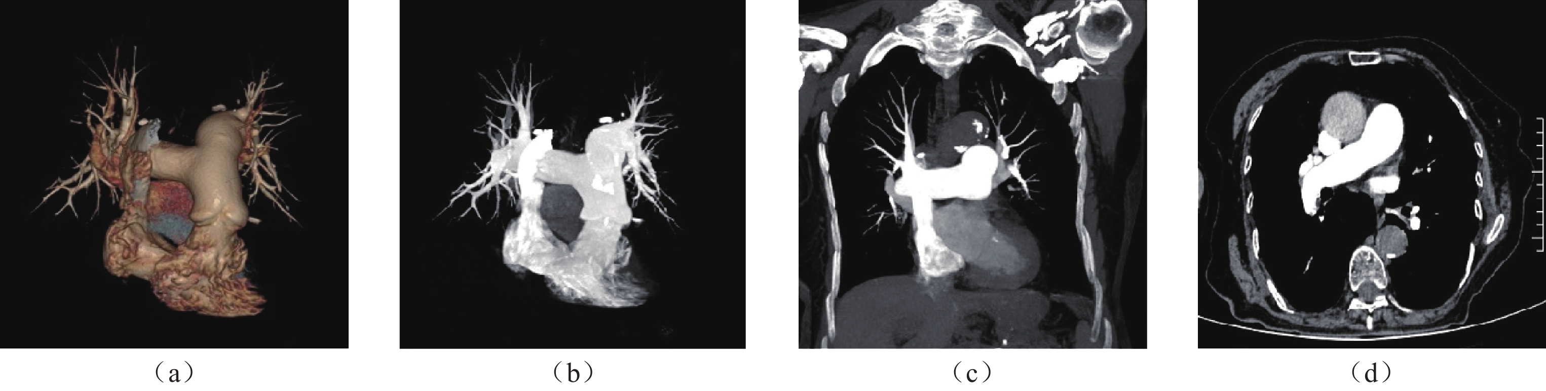
图 1 A组注射方案的VR、MIP、MPR及横断位图
注:患者体重:60 kg,对比剂总量:36 mL,注射流速:3.6 mL/s。图像显示:肺动脉主干、左右动脉及其第5~6级细小肺动脉血管显示清晰,5分;上腔静脉内见少量对比剂潴留,横断位上腔静脉内对比剂有放射状伪影-1分,综合评分:4分。
Figure 1. VR, MIP, MPR, and cross-sectional map of injection regimen of Group A
![]()
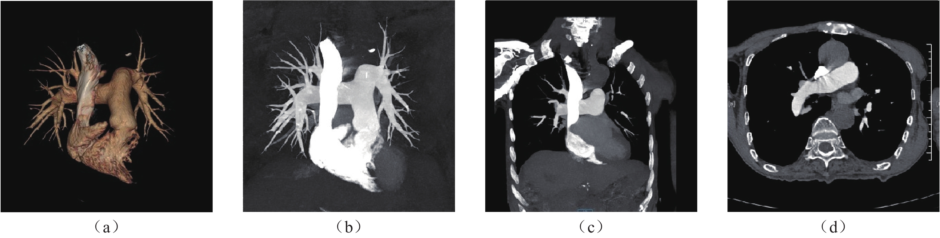
图 2 B组注射方案的VR、MIP、MPR及横断位图
注:患者体重:63 kg,对比剂总量:30 mL,注射流速:3.8 mL/s。图像显示:肺动脉主干、左右动脉及其第5~6级细小肺动脉血管显示清晰,评分5分,上腔静脉内见密度较淡对比剂,横断位上腔静脉内对比剂未见放射状伪影,0分,综合评分:5分。
Figure 2. VR, MIP, MPR, and cross-sectional map of injection regimen of Group B
表 1 两组不同时长的个性化注射方案的一般情况比较
Table 1 General comparison of two personalized injection regimens with different durations
项目 组别 统计检验 A组 B组 t P 男/女 23/31 29/23 2.77 0.74 年龄/Y 68.94±17.99 71.10±12.84 0.73 0.67 身高/mm 165.70± 8.24 166.98± 8.80 2.25 0.07 体重/kg 62.61±10.57 65.62±12.83 0.58 0.10 肺栓塞阳性/阴性 13/41 11/41 0.23 0.32  下载: 导出CSV
表 2 两组不同注射方案的图像质量比较
Table 2 Comparison of image quality between two different injection schemes
指标 分组 统计检验 A组 B组 t P 注射总量 40.74±4.43 34.42±3.05 4.13 0.01 注射时长 10.00±0.00 8.00±0.00 7.37 0.00 注射速度 4.07±0.44 4.10±0.37 12.63 0.06 上腔静脉CT值 740.02±542.05 460.54±211.20 7.60 0.00 肺动脉主干CT值 388.41±79.06 368.21±81.23 0.20 0.88 右肺动脉CT值 357.56±72.35 358.92±93.47 0.41 0.10 左肺动脉CT值 361.96±71.46 358.29±95.23 0.84 0.10 左房CT值 175.06±73.78 196.13±69.39 2.85 0.46 图像主观评分 4.12±0.74 4.59±0.73 1.77 0.04
下载: 导出CSV
-
[1] BARCO S, MAHMOUDPOUR S H, VALERIO L, et al. Trends in mortality related to pulmonary embolism in the European Region, 2000-15: analysis of vital registration data from the WHO Mortality Database[J]. Elsevier, 2020(3): 277-287. DOI: 10.1016/s2213-2600(19)30354-6.
[2] BARCO S, VALERIO L, AGENO W, et al. Age-sex specific pulmonary embolism-related mortality in the USA and Canada, 2000-18: An analysis of the WHO mortality database and of the CDC multiple cause of death database[J]. The Lancet. Respiratory medicine, 2021, 9(1): 33-42. DOI: 10.1016/S2213-2600(20)30417-3.
[3] KONSTANTINIDES S V, MEYER G, BECATTINI C, et al. 2019 ESC Guidelines for the diagnosis and management of acute pulmonary embolism developed in collaboration with the European Respiratory Society (ERS)[J] European Heart Journal, 2020, 41(4): 543-603. doi: 10.1093/eurheartj/ehz405.
[4] KONSTANTINIDES SV, TORBICKI A, AGNELLI G, et al. 2014 ESC Guidelines on the diagnosis and management of acute pulmonary embolism[J]. European Heart Journal, 2015, 35(43): 3033-3069. DOI: 10.1093/eurheartj/ehu283.
[5] PALM V, RENGIER F, RAJIAH P, et al. Acute pulmonary embolism: Imaging techniques, findings, endovascular treatment and differential diagnoses[J]. RoFo: Fortschritte auf dem Gebiete der Rontgenstrahlen und der Nuklearmedizin, 2020, 192(1): 38-49. DOI: 10.1055/a-0900-4200.
[6] RATNAKANTHAN P J, KAVNOUDIAS H, PAUL E, et al. Weight-adjusted contrast administration in the computed tomography evaluation of pulmonary embolism[J]. Journal of Medical Imaging and Radiation Sciences, 2020, 51(3). DOI: 10.1016/j.jmir.2020.06.002.
[7] MCCULLOUGH P A, CHOI J P, FEGHALI G A, et al. Contrast-induced acute kidney injury[J]. Journal of the American College of Cardiology, 2016, 68(13): 1465-1473 DOI: 10.1016/j.jacc.2016.05.099.
[8] 王永胜, 王晨思, 陆浩宇, 等. 个性化造影剂注射方案在提升肺动脉CTA生物应用安全性的价值研究[J]. CT理论与应用研究, 2021, 30(6): 777-783. WANG Y S, WANG C S, LU H Y, et al. Study on the value of individualized contrast agent injection scheme in improving the biosafety of pulmonary Artery CTA[J]. CT Theory and Applications, 2021, 30(6): 777-783. (in Chinese).
[9] 罗立峰, 田丰, 王俊鹏, 等. 应用低剂量对比剂肺动脉CTA成像检查肺动脉栓塞的可行性研究[J]. 中国CT和MRI杂志, 2022, 20(1): 79-81. DOI: 10.3969/j.issn.1672-5131.2022.01.025. LUO W F, TIAN F, WANG J P, et al. Feasibility Study of Pulmonary Artery CTA Imaging with Low-Dose Contrast Agent for Pulmonary Embolismg[J]. Chinese Journal of CT and MRI, 2022, 20(1): 79-81. DOI: 10.3969/j.issn.1672-5131.2022.01.025. (in Chinese).
[10] 王永胜, 杨磊清, 杨怡帆, 等. 不同触发阈值对肺动脉CTA图像质量影响的研究[J]. CT理论与应用研究(中英文), 2024, 33(2): 175-181. DOI: 10.15953/j.ctta.2023.121. WANG Y S, YANG L Q, YANG Y F, et al. The effect of different trigger thresholds on the quality of pulmonary artery CT angiography images[J]. CT Theory and Applications, 2024, 33(2): 175-181. DOI: 10.15953/j.ctta.2023.121.
[11] ZHANG F F, LU Z Y, WANG F. Advances in the pathogenesis and prevention of contrast-induced nephropathy[J]. Life Sciences, 2020, 259(6): 118379. DOI: 10.1016/j.lfs.2020.118379.
[12] 谢希, 杨春静, 范菁. 肺动脉CT血管造影扫描最佳碘对比剂注射方案的应用研究[J]. 临床医药实践, 2023, 32(1): 47-50. XIE X, YANG C J, FAN J. Application standy of optimal iodine econtrast medium injection scheme in pulmonary Artery CTA scans[J]. Proceeding of Clinical Medicine, 2023, 32(1): 47-50. (in Chinese).
[13] LISELOTTE V D P, TROMEUR C, FABER L, et al. Chest X-ray not routinely indicated prior to the years algorithm in the diagnostic management of suspected pulmonary embolism[J]. Th Open, 2021, 3(1): 22-27.
[14] JAMALI L, ALIKHANI B, GETZIN T, et al. Arterial attenuation in individualized computed tomography pulmonary angiography injection protocol adjusted based on the patient's body mass index[J]. Journal of Research in Medical Sciences, 2020, 25: 94. DOI: 10.4103/jrms.JRMS_690_19.
[15] SILVAL M, MILANESE G, COBELLI R et al. CT angiography for pulmonary embolism in the emergency department: Investigation of a protocol by 20mL of high-concentration contrast medium[J]. La Radiologia Medica, 2020, 125(2): 137-144. DOI: 10.1007/s11547-019-01098-6.
[16] 王素丽, 孙莉薇, 刘丹妮, 等. 个性化扫描方案应用于肺动脉CT血管造影扫描中的价值分析[J]. 现代医用影像学, 2022, 37(3): 31-35. DOI: 10.3969/j.issn.1006-7035.2022.3.xdyyyxx202203034. WANG S L, SUN L W, LIU D N, et al. Value analysis of personalized scanning scheme applied in pulmonary artery CT angiography scanning[J]. Modern Medical Imageology, 2022, 37(3): 31-35. DOI: 10.3969/j.issn.1006-7035.2022.3.xdyyyxx202203034. (in Chinese).


计量
- 文章访问数: 41
- HTML全文浏览量: 18
- PDF下载量: 3
