Computed Tomography Reconstruction Algorithm Based on Relative Total Variation Minimization
-
摘要: 总变差(TV)最小算法是一种有效的CT图像重建算法,可以对稀疏或含噪投影数据进行高精度重建。然而,在某些情况下,TV算法会产生阶梯状伪影。在图像去噪领域,相对TV算法展现了优于TV算法的性能。鉴于此,将相对TV模型引入图像重建,提出相对TV最小优化模型,并在自适应梯度下降-投影到凸集(ASD-POCS)框架下设计对应的求解算法,以进一步提升重建精度。以Shepp-Logan、FORBILD及真实CT图像仿真模体进行重建实验,验证了该算法的正确性并评估了算法的稀疏重建能力和抗噪能力。实验结果表明,相对TV算法可以实现逆犯罪,可以对稀疏或含噪投影数据进行高精度重建,与TV算法相比,该算法可以取得更高的重建精度。
-
关键词:
- 计算机断层成像 /
- 相对总变差最小 /
- 稀疏重建 /
- ASD-POCS算法
Abstract: The total variation (TV) minimization algorithm is an effective CT image reconstruction algorithm that can reconstruct sparse or noisy projection data with high accuracy. However, in some cases, the TV algorithm produces stepped artifacts. The relative TV algorithm outperforms TV algorithm in the field of image denoising. In view of this, the relative TV model is introduced into image reconstruction, a relative TV minimum optimization model is proposed, and the corresponding solution algorithm is designed under the framework of adaptive gradient descent projection to the convex set (ASD-POCS) to further improve reconstruction accuracy. The reconstruction experiments were conducted with Shepp Logan, Forbild, and real CT image simulation models to verify the anti-crime ability of the algorithm and evaluate the sparse reconstruction and anti-noise abilities of the algorithm. The experimental findings reveal that the algorithm outperforms the TV method in terms of anti-crime capability and the ability to reconstruct sparse or noisy projection data with high precision. Compared with the TV algorithm, the algorithm can achieve higher reconstruction accuracy. -
计算机断层成像(computed tomography,CT)、磁共振成像(magnetic resonance imaging,MRI)、电子顺磁共振成像(electron paramagnetic resonance imaging,EPRI)是3种重要的医学成像模态。在CT成像中,以滤波反投影(filtered back projection,FBP)算法[1]为代表的解析法是一类经典的医学图像重建算法,其重建速度快、精度高。然而,当投影数据不完备时,其在成像中可能会产生严重的伪影[2-3]。对于这个问题,一种解决方法是利用插值对稀疏投影数据进行补足,另一种方法是Sidky等[2]在2008年提出的一种经典的迭代式重建算法,即总变差(total variation,TV)最小化算法[4],它通过加入先验的知识来正则化对应的数据保真项,可以在去噪的同时保持图像的边缘信息[5],实现了在稀疏投影数据下的高精度图像重建。随后,Sidky等[6]进一步优化了该算法,提出了自适应最速下降投影到凸集(adaptive gradient descent projection to convex set,ASD-POCS)算法并以之作为该算法的有效求解器。
此后有大量的TV模型及对应的求解算法[7-8]被提出。2014年,Sidky等[9]提出了约束总p变差(total p variation,TpV)模型并利用CP(chambolle-pock)优化算法[10-12]求解该模型,在稀疏投影数据条件下实现了高精度的图像重建;2012年,Xu等[13]提出了相对总变差(relative total variation,RTV)模型,此模型最初是应用于图像去噪,可以从不规则的纹理中提取出有效的结构信息,借助于对噪声和不规则纹理的去除能力可以应用于CT重建;2015年,Rigie等[14]提出了多通道光谱CT的总核变差(total nuclear variation,TnV)模型,发现这种联合TV正则化技术优于每个通道的单独TV最小化;2021年Qiao等[15]提出了平衡总变差(balanced total variation,bTV)模型,可以在三维电子顺磁共振成像(EPRI)应用[5]中保证收敛并实现快速收敛。其他优秀的重建模型还有,高阶总变差(high order TV,HOTV)[16]、各向异性总变差(anisotropic TV,aTV)[17]等等,这些TV模型在投影数据不完整时,在一定程度上都可以提高重建精度。
综合研究发现,这些TV模型的改进都是尝试去解决TV模型的潜在缺点,即TV模型在重建过程中可能会产生条状伪影[6]。主要原因是图像的总变差(TV)是图像梯度的11范数[18],在图像TV最小化[19]的过程中,重建图像中的所有梯度都会受到类似的惩罚,这对于保护图像的有效结构是不利的。图像梯度的10范数用于计算图像中非零梯度的个数,不会对梯度进行求和,所以如果对重建图像梯度的10范数进行最小化,重建图像中梯度较大的结构不会受到过度的惩罚,相对来说有利于保护图像结构。然而,却可能会平滑掉梯度较小的图像结构,不利于保留图像细节。同时,在稀疏投影数据下的重建过程中,有一些噪声的梯度可能和较小图像结构的梯度是一样,此时重建图像梯度的10范数最小化并不能有效地抑制噪声。
考虑到图像梯度11范数和10范数最小化的缺点,在CT重建过程中应该考虑对不同大小的图像梯度进行不同程度的惩罚,以此来保护有效结构并抑制噪声。此外,为了防止梯度较小的图像结构在重建中被平滑掉,可以考虑把图像梯度大小的信息作为先验知识引入到重建模型中。
我们发现RTV可以通过其定义的一种巧妙的窗口固有变差(windowed inherentvariation,WIV)来对不同大小的图像梯度进行不同程度的惩罚,借此来将其应用到CT重建中。具体来讲,对于某个像素点,如果以这个像素点为中心的窗口区域内的像素点的偏导数的符号相对一致,即如果这个区域内的有效结构较多,那么这个像素点的WIV值相对会比较大。反之,如果以这个像素点为中心的窗口区域内的像素点的偏导数的符号是随机的,那么这个区域内的噪声往往会比较多,其WIV值相对会比较小。所以,WIV值会作为惩罚权重在稀疏投影CT重建中自适应地保护图像结构并抑制噪声,在精确重建图像结构信息的同时梯度较小的图像结构也能得到有效的保护。
鉴于上述RTV模型的优点,我们可以将其应用到CT重建中,提出RTV最小化算法以实现RTV图像重建,并在ASD-POCS框架下设计对应的求解算法,通过Shepp-Logan、FORBILD[20]和真实CT图像模体进行仿真实验,来验证该算法的正确性,评估其稀疏重建和去噪的能力。
1. 相关知识
1.1 成像模型
本文以二维平行束CT重建作为研究对象。离散-离散(discrete to discrete,D2D)的成像模型把投影和图像都作为离散数据。则平行束CT的成像模型能够被表示为如下线性方程组:
$$ {{\boldsymbol{g}} = {\boldsymbol{Af}}} \text{,} $$ (1) 其中,f是一个大小为N的的列向量,表示离散图像;g是一个大小为M的列向量,表示离散投影数据;A是一个大小为
$M \times N$ 的系统矩阵,这里代表2D Radon变换;${A_{m,n}}$ 表示第n个像素对第m个投影测量值的贡献。实际上,求取系统矩阵
${{{A}}_{m,n}}$ 的方法相当于是投影方法。本文系统矩阵采用Siddon射线驱动法[21]求取。因此,对于2D Radon变换来说,${A_{m,n}}$ 表示第n个像素与第m条射线的相交长度。假设图像的大小是
${n_x} \times {n_y}$ ,将其按列串行化,从而使用向量对图像进行表示,其大小为$N = {n_x} \times {n_y}$ 。假设投影的大小是${n_i} \times {n_j}$ ,这表示在${n_i}$ 个角度下进行投影,而每个角度下的投影向量有${n_j}$ 个投影值,将其按列进行串行化,就可以得到投影数据的向量表示,其大小为$M = {n_i} \times {n_j}$ 。一般情况下,系统矩阵是非常庞大的、欠定的、甚至是病态的,因此线性方程组(1)无法通过对其直接求逆来得到最优解,所以为获了得更高的重建精度,需进一步将此模型建模为一个最优化问题来进行求解。
1.2 TV最小化重建模型
根据上述成像模型,对于离散图像f约束的TV最优化模型可表示为:
$$ {{{\boldsymbol{f}}^*} = {\rm{arg}}\mathop {\min}\limits_{\boldsymbol{f}} {{\big\| {\boldsymbol{f}} \big\|}_{{\text{TV}}}}\quad {\rm{s}}.{\rm{t}}.\quad{{\big\| {{\boldsymbol{g}} - {\boldsymbol{Af}}} \big\|}_2} \leq \varepsilon } \text{,} $$ (2) 式中,
${{\boldsymbol{f}}^*}$ 表示的是最优化模型的解,即被重建的图像;${\big\| {\boldsymbol{f}} \big\|_{{\text{TV}}}}$ 表示的是图像f的${\text{TV}}$ 范数,也就是图像梯度大小变换${\left| {{\boldsymbol{Df}}} \right|_{{\rm{mag}}}}$ 的11范数,如等式(3)所示;${\big\| {{\boldsymbol{g}} - {\boldsymbol{Af}}} \big\|_2}$ 是数据保真项,表示的是生成投影数据与实际测量投影值数据之间的差异的12范数;$\varepsilon $ 为数据容差,与噪声水平有关。$$ {{{\big\| {\boldsymbol{f}} \big\|}_{{\text{TV}}}} = {{\big\| {{{\left| {{\boldsymbol{Df}}} \right|}_{{\rm{mag}}}}} \big\|}_1}} 。 $$ (3) 在等式(3)中D是一个大小为
$2 N \times N$ 的矩阵:$$ {{\boldsymbol{D}} = \left( {\begin{array}{*{20}{c}} {{{\boldsymbol{D}}_{\boldsymbol{x}}}} \\ {{{\boldsymbol{D}}_{\boldsymbol{y}}}} \end{array}} \right)} \text{,} $$ (4) 其中,
${{\boldsymbol{D}}}_{x}和{{\boldsymbol{D}}}_{y}$ 均为$N \times N$ 的矩阵,分别表示沿着x和y轴方向的离散梯度变换。令
$ {u}_{x,y},x\in \left[1,{n}_{x}\right] $ ,$y \in \left[ {1,{n_y}} \right]$ 表示二维图像的每个像素,则${{\boldsymbol{{\boldsymbol{D}}}}_x}{\boldsymbol{f}}$ ,${D_y}{\boldsymbol{f}}$ 可以表示为:$$ {\Big({{\boldsymbol{D}}}_{x}{\boldsymbol{f}}\Big)}_{x,y}=\left\{ \begin{array}{ccl}&{{\boldsymbol{f}}}_{x,y}-{{\boldsymbol{f}}}_{x-1,y}\text{,}& x\in \left[2,{n}_{x}\right]\\ &0\text{,}& x=1\end{array}\right. \text{,} $$ (5) $$ {\Big({{\boldsymbol{D}}}_{y}{\boldsymbol{f}}\Big)}_{x,y}=\left\{ \begin{array}{ccl} &{{\boldsymbol{f}}}_{x,y}-{{\boldsymbol{f}}}_{x,y-1}\text{,}& {y}\in \left[2,{n}_{y}\right]\\ &0\text{,}& y=1\end{array}\right. 。 $$ (6) 令
${\left| {{\kern 1 pt} \cdot {\kern 1 pt} } \right|_{{\rm{mag}}}}$ 表示对一个二维向量求模,可以是11范数模,也可以是12范数模。本文中,采用12范数模,即:$$ {{{\bigg\| {\begin{array}{*{20}{c}} {{\kern 1pt} a{\kern 1pt} } \\ {{\kern 1pt} b{\kern 1pt} } \end{array}} \bigg\|}_{{\rm{mag}}}} = {{\bigg\| {\begin{array}{*{20}{c}} {{\kern 1pt} a{\kern 1pt} } \\ {{\kern 1pt} b{\kern 1pt} } \end{array}} \bigg\|}_2} = \sqrt {{a^2} + {b^2}} } 。 $$ (7) 这样
${\big\| {\boldsymbol{f}} \big\|_{{\text{TV}}}}$ 可以被表示为:$$ {\big\| {\boldsymbol{f}} \big\|_{_{{\text{TV}}}}} = {\big\| {{\boldsymbol{Df}}} \big\|_{{\text{mag1}}}} = \mathop \sum \limits_{x,y} \sqrt {{{\left( {{{\boldsymbol{f}}_{x,y}} - {{\boldsymbol{f}}_{x - 1,y}}} \right)}^2} + {{\left( {{{\boldsymbol{f}}_{x,y}} - {{\boldsymbol{f}}_{x,y - 1}}} \right)}^2}} 。 $$ (8) 1.3 RTV模型
作为TV模型的一种改进形式,RTV的定义[13]如下:
$$ {{\text{RTV}}\left( {{{\boldsymbol{f}}_p}} \right) = \lambda \cdot \left( {\frac{{{\mathcal{D}_x}\left( {{{\boldsymbol{f}}_p}} \right)}}{{{\mathcal{L}_x}\left( {{{\boldsymbol{f}}_p}} \right) + \varepsilon }} + \frac{{{\mathcal{D}_y}\left( {{{\boldsymbol{f}}_p}} \right)}}{{{\mathcal{L}_y}\left( {{{\boldsymbol{f}}_p}} \right) + \varepsilon }}} \right)} \text{,} $$ (9) 式中,λ表示权重,
${\mathcal{D}_x}\left( p \right)$ 和${\mathcal{D}_y}\left( p \right)$ 是窗口总变差(windowed total variation,WTV),其定义如下:$$ {{\mathcal{D}_x}\left( {{{\boldsymbol{f}}_p}} \right) = \mathop \sum \limits_{q \in \mathcal{W}\left( p \right)} {h_{p,q}} \cdot \left| {{{\left( {{\partial _x}{\boldsymbol{f}}} \right)}_q}} \right|} \text{,} $$ (10) $$ {{\mathcal{D}_y}\left( {{{\boldsymbol{f}}_p}} \right) = \mathop \sum \limits_{q \in \mathcal{W}\left( p \right)} {h_{p,q}} \cdot \left| {{{\left( {{\partial _y}{\boldsymbol{f}}} \right)}_q}} \right|} 。 $$ (11) x和y表示方向;
$\mathcal{W}\left( p \right)$ 表示的是一个以图像f的第p个像素点为中心的局部矩形区域,q是这个矩形区域内的像素索引,${h_{p,q}}$ 表示的是以σ为标准差的高斯函数。而${\mathcal{L}_x}\left( p \right)$ 和${\mathcal{L}_y}\left( p \right)$ 表示的是窗口固有变差(WIV),其定义如下:$$ {{\mathcal{L}_x}\left( {{{\boldsymbol{f}}_p}} \right) = \left| {\mathop \sum \limits_{q \in \mathcal{W}\left( p \right)} {h_{p,q}} \cdot {{\left( {{\partial _x}f} \right)}_q}} \right|} \text{,} $$ (12) $$ {{\mathcal{L}_y}\left( {{{\boldsymbol{f}}_p}} \right) = \left| {\mathop \sum \limits_{q \in \mathcal{W}\left( p \right)} {h_{p,q}} \cdot {{\left( {{\partial _y}f} \right)}_q}} \right|} 。 $$ (13) 将等式(10)~等式(13)代入等式(9)进行推导可得RTV范式的矩阵表达形式:
$$ {{{\big\| {\boldsymbol{f}} \big\|}_{{\text{RTV}}}} = \lambda \cdot \left( {{\boldsymbol{V}}_{\boldsymbol{f}}^{\rm{T}}{\boldsymbol{C}}_{\boldsymbol{f}}^{\rm{T}}{{\boldsymbol{U}}_{\boldsymbol{x}}}{{\boldsymbol{Z}}_{\boldsymbol{x}}}{{\boldsymbol{C}}_{\boldsymbol{x}}}{{\boldsymbol{V}}_{\boldsymbol{f}}} + {\boldsymbol{V}}_{\boldsymbol{f}}^{\rm{T}}{\boldsymbol{C}}_{\boldsymbol{y}}^{\rm{T}}{{\boldsymbol{U}}_{\boldsymbol{y}}}{{\boldsymbol{Z}}_{\boldsymbol{y}}}{{\boldsymbol{C}}_{\boldsymbol{y}}}{{\boldsymbol{V}}_{\boldsymbol{f}}}} \right)} \text{,} $$ (14) 其中λ表示权重,
${{\boldsymbol{V}}_{\boldsymbol{f}}}$ 表示重建图像的向量表示,${{\boldsymbol{C}}_{\boldsymbol{x}}}$ 和${{\boldsymbol{C}}_{\boldsymbol{y}}}$ 表示向前差分近似的离散梯度算子得到的Toeplitz矩阵。${{\boldsymbol{U}}_{\boldsymbol{x}}}$ ,${{\boldsymbol{U}}_{\boldsymbol{y}}}$ ,${{\boldsymbol{Z}}_{\boldsymbol{x}}}$ ,${{\boldsymbol{Z}}_{\boldsymbol{y}}}$ 均为对角矩阵。上述详细推导过程可以参考Xu等[13]发表的相关研究。
2. 本文方法
2.1 RTV最小化重建模型
本文方法主要受文献[2]和文献[13]的启发,2008年Sidky等[2]提出ASD-POCS算法,应用正则化方法将目标函数定义为优化准则与惩罚项之和的形式,以罚函数的形式增强解的稳定性。ASD-POCS算法改进于Sidky等[6]于2006年提出的重建算法,2006年的算法首次结合医学图像的梯度变换图像具有稀疏性这一先验知识,利用凸集投影,使得ART等迭代算法在稀疏投影数据的条件下,相较于FBP等解析类算法表现出极为精确的重建能力。
然而在ASD-POCS算法所对应的TV最小化重建模型中,TV范数是图像梯度的11范数,由等式(8)可知,在TV最小化的过程中,会对重建图像的所有梯度施加惩罚,在重建过程中可能会出现伪影。所以,在重建过程中应该考虑对重建图像不同大小的梯度施加不同的惩罚,这样可以更好的区分图像结构和噪声,达到保护图像并抑制噪声的目的。
2012年,Xu等[13]提出RTV模型,可以通过其所定义WIV有效的区分噪声和图像结构。因此,针对ASD-POCS算法中TV最小化的缺点,鉴于RTV对噪声和不规则纹理的去除能力,我们选择使用RTV模型来约束最终解,将RTV作为正则项引入到CT重建模型中,使用梯度下降法来求解RTV最小化。
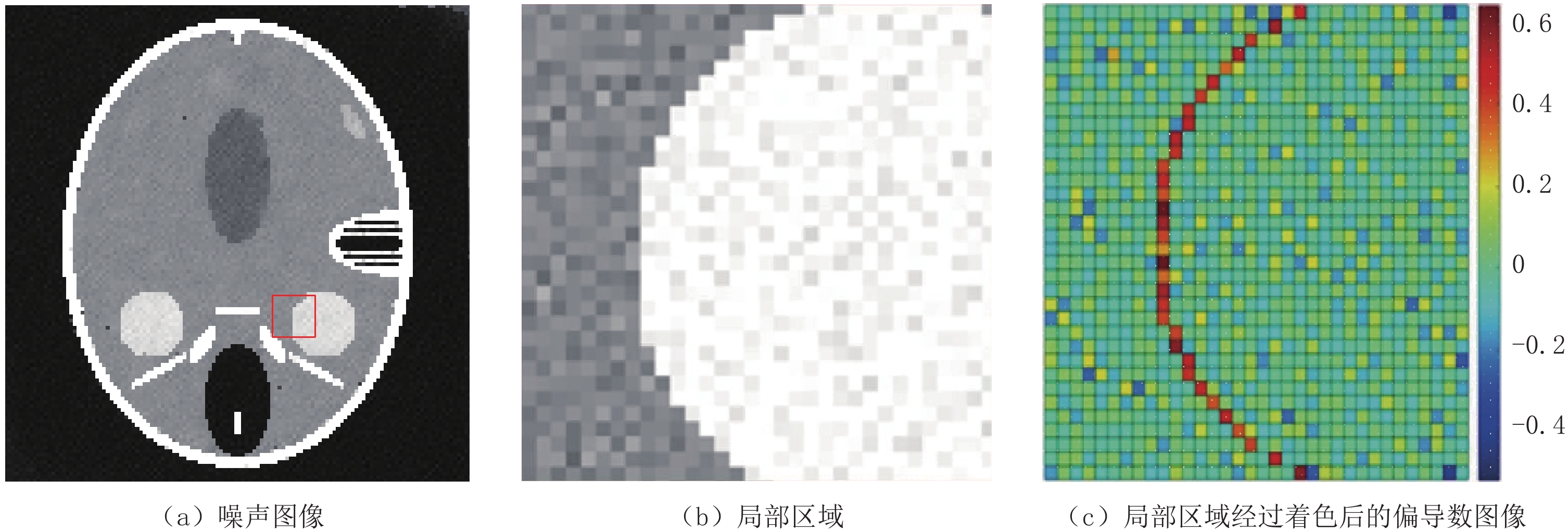
那么,当重建图像含有明显的噪声时,RTV最小化是否可以有效地区分重建图像中的结构和噪声?一个重要的先验知识是:在含噪图像中,图像有效结构处的偏导数往往具有相同的符号,而含有更多噪声区域内偏导数的符号往往是随机的。如图1所示:图1(a)是一幅含有明显噪声的重建图像;图1(b)是其中局部矩形区域的放大图;图1(c)是局部区域在着色后的偏导数图像。借此来说明含噪重建图像像素偏导数的特点,其中不同颜色代表不同大小的偏导数的值。可见,重建图像有效结构处偏导数的绝对值偏大并且大多数具有相同的符号,而含有更多噪声区域内偏导数的符号往往是随机的。
进一步从等式(10)和等式(12)可见,WTV首先是取偏导数的绝对值,然后再取偏导数的加权和。而WIV是首先取偏导数的加权和再取绝对值。对于WIV来说,由于图像f在局部矩形区域
$\mathcal{W}\left( p \right)$ 内任一点的偏导数有正负两种情况,所以直接求和会产生数值上的抵消。这样,对于包含更多噪声的局部矩形区域内的WIV值来说,这个区域内像素点的偏导数的符号往往是随机的,所以其加权和自然要小于包含更多有效结构的局部矩形区域内的WIV值。通过这样的方式,WIV作为惩罚权重可以在稀疏投影重建中自适应地保护图像结构和抑制噪声并且准确的重建图像结构。通过前文对RTV的分析可知,RTV最小化能够被使用在CT重建中,并且可以在很大程度上保护图像结构并抑制噪声。所以为了在稀疏角度下更精确地进行图像重建,本文在TV算法的基础上进行了改进。把RTV作为正则项引入至CT重建模型中,提出RTV最小化图像重建模型,其定义如下:
$$ {{{\boldsymbol{f}}^{\boldsymbol{*}}} = {\rm{arg}}\mathop {\min}\limits_{{\boldsymbol{f}} \geq 0} {{\big\| {\boldsymbol{f}} \big\|}_{{\text{RTV}}}}\quad {\rm{s.t}}.\quad{{\big\| {{\boldsymbol{g}} - {\boldsymbol{Af}}} \big\|}_2} \leq \in } \text{,} $$ (15) 其中,
${{\boldsymbol{f}}^{\boldsymbol{*}}}$ 表示重建图像;$ {\big\| {\boldsymbol{f}} \big\|_{{\text{RTV}}}} $ 为正则项,作用是抑制噪声并保护图像结构;$f \geq 0$ 保证体素值不为负。${\big\| {\boldsymbol{f}} \big\|_{{\text{RTV}}}}$ 的定义如等式(14)所示,其导数计算如下:$$ {{\nabla _f}{{\big\| {\boldsymbol{f}} \big\|}_{_{{\text{RTV}}}}} = \frac{{\partial {\text{RTV(}}{\boldsymbol{f}}{\text{)}}}}{{\partial {\boldsymbol{f}}}}} = {2\lambda \cdot \left( {{\boldsymbol{C}}_{\boldsymbol{f}}^{\rm{T}}{{\boldsymbol{U}}_{\boldsymbol{x}}}{{\boldsymbol{Z}}_{\boldsymbol{x}}}{{\boldsymbol{C}}_{\boldsymbol{x}}} + {\boldsymbol{C}}_{\boldsymbol{y}}^{\rm{T}}{{\boldsymbol{U}}_{\boldsymbol{y}}}{{\boldsymbol{Z}}_{\boldsymbol{y}}}{{\boldsymbol{C}}_{\boldsymbol{y}}}} \right){{\boldsymbol{V}}_{\boldsymbol{f}}}} 。 $$ (16) 该模型可以在ASD-POCS框架[6]下进行求解,ASD-POCS框架是一个迭代框架,每一次迭代大体可分为两个步骤:凸集投影和梯度下降操作。凸集投影(POCS)操作就是代数重建技术(algebraic reconstruction technique,ART)[22]操作,可以减小真实投影g和重建图像的模拟投影Af之间的差距,满足数据保真项约束;梯度下降操作是通过自适应步长使用最速下降法,实现RTV最小化。具体步骤如下:
(1)参数初始化,参数包括:RTV最速下降迭代次数
${N_{{\rm{grad}}}}$ ,RTV正则项权重参数λ,用于控制RTV正则项的强度、RTV正则项参数ε,避免分母为0的情况出现,参数σ,用于控制WTV、WIV矩形区域空间比例、ART算法迭代松弛因子${\beta _{{\rm{red}}}}$ 、RTV最速下降迭代松弛因子${\alpha _{{\rm{red}}}}$ 、${r_{{\rm{max}}}}$ 、数据容差$ \in $ ,重建图像初始值${{\boldsymbol{f}}^{{\text{(0)}}}}$ 。(2)使用ART算法,经过迭代得到满足数据一致性约束的图像
${{\boldsymbol{f}}^{(n)}}$ :$$ {{\boldsymbol{f}}^{(n)}} = {{\boldsymbol{f}}^{(n - 1)}} + {\beta _{{\rm{red}}}}{{\boldsymbol{A}}_i}\frac{{{g_i} - {{\boldsymbol{A}}_i}{\boldsymbol{ \times }}{{\boldsymbol{f}}^{(n - 1)}}}}{{{{\boldsymbol{A}}_i}{\boldsymbol{ \times }}{{\boldsymbol{A}}_j}}},\quad\;\;i,j = 1,2, \cdots ,N。 $$ (3)更新
${{\boldsymbol{f}}^{{{(n)}}}}$ ,使重建图像满足非负约束限制:$$ {\boldsymbol{f}}_j^{{\text{(}}n{\text{)}}} = \left\{ \begin{aligned} & {\boldsymbol{f}}_j^{(n)},&{\boldsymbol{f}}_j^{(n)} \geq 0 \\ &0,& {\boldsymbol{f}}_j^{(n)} \leq 0 \\ \end{aligned} \right. 。 $$ (4)将满足非负约束条件的
${{\boldsymbol{f}}^{(n)}}$ 作为RTV最速下降迭代的初始值:$$ {\boldsymbol{f}}_{{\text{RTV-GRAD}}}^{(n)} = {{\boldsymbol{f}}^{(n)}} 。 $$ (5)计算参数:
$ \nabla {{\boldsymbol{f}}_{{\text{POCX}}}} = {\big\| {{{\boldsymbol{f}}^{(n)}} - {{\boldsymbol{f}}^{(n - 1))}}} \big\|_2} $ ,$ {d_\alpha } = \alpha \cdot \nabla {{\boldsymbol{f}}_{{\text{POCX}}}} $ ,${\boldsymbol{\hat g}} = {\boldsymbol{A}} \times {\boldsymbol{f}}$ ,$ {d_p} = {\big\| {{\boldsymbol{\hat g - }}{{\boldsymbol{g}}_{\boldsymbol{0}}}} \big\|_2} $ 。(6)RTV最速下降迭代:
$$ {{\nabla _f}{{\big\| {{{\boldsymbol{f}}^{(n)}}} \big\|}_{_{{\text{RTV}}}}}^{(k)} = \frac{{\partial {\text{RTV}}\left( {{{\boldsymbol{f}}^{(n)}}} \right)}}{{\partial {{\boldsymbol{f}}^{(n)}}}}} \text{,} $$ $$ {\boldsymbol{f}}_{{\text{RTV-GRAD}}}^{(n)} = {\boldsymbol{f}}_{{\text{RTV-GRAD}}}^{(n)} - {d_\alpha }\frac{{{\nabla _f}{{\big\| {{{\boldsymbol{f}}^{(n)}}} \big\|}_{_{{\text{RTV}}}}}^{(k)}}}{{\big\| {{\nabla _f}{{\big\| {{{\boldsymbol{f}}^{(n)}}} \big\|}_{_{{\text{RTV}}}}}^{(k)}} \big\|}} 。 $$ (7)更新RTV最速下降迭代参数和ART迭代的松弛因子:
$$ \nabla {{\boldsymbol{f}}_{{\text{RTV}}}} = {\big\| {{\boldsymbol{f}}_{{\text{RTV-GRAD}}}^{(n)} - {{\boldsymbol{f}}^{(n)}}} \big\|_2} 。 $$ 更新RTV最速下降迭代松弛因子和RTV正则项权重参数:
$$ \alpha = \left\{ \begin{gathered} \alpha \cdot {\alpha _{{\rm{red}}}},\;\quad{\rm{if}}{\text{ }}\nabla {{\boldsymbol{f}}_{{\text{TV}}}} \geq {r_{\max}} \cdot \nabla {{\boldsymbol{f}}_{{\text{POCX}}}}{\text{ }}{\rm{and}}{\text{ }}{d_p} \geq \in \\ \alpha ,\quad\qquad\;{\rm{others}} \\ \end{gathered} \right.。 $$ 更新ART迭代松弛因子:
$$ \beta = \beta \cdot {\beta _{{\rm{red}}}}。 $$ 如果满足迭代停止条件,则返回
${\boldsymbol{f}}_{{\text{RTV-GRAD}}}^{(n)}$ ,否则令${{\boldsymbol{f}}^{(n)}} = {\boldsymbol{f}}_{{\text{RTV-GRAD}}}^{(n)}$ ,转到步骤(2)继续计算。以上,步骤(2)和步骤(3)这两步是凸集投影和非负约束操作,保证数据的一致性和非负性;步骤(4)到步骤(7)是RTV最小化操作,使得到的最优解不仅满足数据一致性和非负性约束,而且满足RTV最小化。
2.2 RTV最小化重建模型求解算法伪代码
RTV最小化重建模型求解算法的伪代码如算法1所示:
算法1:基于ASD-POCS框架的RTV重建算法
输入:RTV最速下降迭代次数
${N_{{\rm{grad}}}} = $ 4、RTV正则项权重参数$\lambda = $ 0.45,用于控制RTV正则项的强度、RTV正则项参数$\varepsilon =$ 0.02,避免分母为$0 $ 的情况出现、矩形区域空间比例参数$\sigma = $ 0.25、ART算法迭代松弛因子${\beta _{{\rm{red}}}} =$ 0.95、RTV最速下降迭代松弛因子${\alpha _{{\rm{red}}}} = $ 0.98,${r_{\max }} = $ 0.95、数据容差$ \in $ 、重建图像初始值${{\boldsymbol{f}}^{{\text{(0)}}}} = $ 0。输出:重建图像
${{\boldsymbol{f}}_{{\rm{res}}}}$ 。1. Repeat main loop 13. $for{\text{ } }i = 1{\text{:} }{N_{{\rm{grad}}} }{\text{ do RTV - ASD loop} }$: 2. $ {{\boldsymbol{f}}}_{p}={{\boldsymbol{f}}}^{(n)}$ ${\boldsymbol{d} }{ {\boldsymbol{f} }^{(k)} } = {\nabla _f}\left\| { { {\boldsymbol{f} }^{(n)} } } \right\|_{{\rm{RTV}}}^{(k)}$ 3. ${\text{for } }i = 1{\text{ : } }{N_d}{\text{ do } }{\boldsymbol{f} } = {\boldsymbol{f} } + \beta { {\boldsymbol{A} }_{\boldsymbol{i} } }\displaystyle \frac{ { {g_i} - { {\boldsymbol{A} }_{\boldsymbol{i} } }{\boldsymbol{ \times f} } } }{ { { {\boldsymbol{A} }_{\boldsymbol{i} } }{\boldsymbol{ \times } }{ {\boldsymbol{A} }_{\boldsymbol{j} } } } }$ $ {\boldsymbol{d}}{{\boldsymbol{f}}^{(k)}} = {{{\boldsymbol{d}}{{\boldsymbol{f}}^{(k)}}} \mathord{\left/ {\vphantom {{{\boldsymbol{d}}{{\boldsymbol{f}}^{(k)}}} {{{\left\| {{\boldsymbol{d}}{{\boldsymbol{f}}^{(k)}}} \right\|}_2}}}} \right. } {{{\left\| {{\boldsymbol{d}}{{\boldsymbol{f}}^{(k)}}} \right\|}_2}}} $ 4. ${\text{for } }i = 1{\text{ : } }{N_i}{\text{ do if } }{{\boldsymbol{f}}_i} < 0{\text{ then } }{{\boldsymbol{f}}_i} = 0$ $ {{\boldsymbol{f}}^{(n)}} = {{\boldsymbol{f}}^{(n)}} - {d_\alpha }*{\boldsymbol{d}}{{\boldsymbol{f}}^{(k)}} $ 5. ${ {\boldsymbol{f} }_{{\rm{res}}} } = { {\boldsymbol{f} }^{(n)} }$ end for 6. ${{\boldsymbol{g}}^{(n)}} = {\boldsymbol{A}} \times {{\boldsymbol{f}}^{(n)}}$ 14. $ \nabla {{\boldsymbol{f}}_{{\text{RTV}}}} = {\left\| {{{\boldsymbol{f}}^{(n)}} - {{\boldsymbol{f}}_p}} \right\|_2} $ 7. ${d_p} = {\left\| {{{\boldsymbol{g}}^{(n)}}{\boldsymbol{ - }}{{\boldsymbol{g}}_{\boldsymbol{0}}}} \right\|_2}$ 15. ${\rm{if}}{\text{ } }\nabla { {\boldsymbol{f} }_{ {\text{RTV} } } } > {r_{\max} }*\nabla { {\boldsymbol{f} }_{ {\text{POCX} } } }{\text{ } }{\rm{and}}{\text{ } }{d_p} > \in {\text{ then} }$ 10. $\nabla {{\boldsymbol{f}}_{{\text{POCX}}}} = {\left\| {{{\boldsymbol{f}}^{(n)}} - {{\boldsymbol{f}}_p}} \right\|_2}$ ${d_\alpha } = {d_\alpha }*{\alpha _{{\rm{red}}} }$ 11. ${\text{if first iterarion , then }}{d_\alpha } = \alpha \cdot \nabla {{\boldsymbol{f}}_{{\text{POCX}}}}$ 16. $\beta = \beta \cdot {\beta _{{\rm{red}}} }$ 12. ${{\boldsymbol{f}}_p} = {{\boldsymbol{f}}^{(n)}}$ 17. ${\text{until}}\left\{ {{\text{stopping criteria}}} \right\}$ 18. ${\text{return } }\;{{\boldsymbol{f}}_{ {\rm{res} } } }$ 其中,
${g_0}$ 是通过Siddon射线驱动法得到的真实投影;${{\boldsymbol{f}}_p}$ 是临时变量,用来储存算法当前步骤的结果并参与步长自适应调整的计算。最外层的每一次迭代主要由POCS和ASD组成,算法的第5~6行执行POCS部分,利用ART操作和正向投影调整数据一致性。算法的第13~17行执行ASD部分,用于实现RTV最小化,算法第14行中图像RTV范式的梯度计算由等式(16)所得。该算法的关键在于如何控制POCS部分和RTV最速下降部分各自的步长。所以通过
$ {d_\alpha } $ 来控制RTV梯度下降的步长,通过控制β的缩放更准确地缩小模拟投影与真实投影间的差距,使得POCS部分与RTV梯度下降部分保持一种平衡。在第10行计算POCS部分引起的图像变化$ \nabla {{\boldsymbol{f}}_{{\text{POCX}}}} $ ,第18行计算梯度下降部分引起的图像变化$ \nabla {{\boldsymbol{f}}_{{\text{RTV}}}} $ ,在第19行执行步长自适应,如果$ \nabla {{\boldsymbol{f}}_{{\text{RTV}}}} $ 和$ \nabla {{\boldsymbol{f}}_{{\text{POCX}}}} $ 的比率大于${r_{{\rm{max}}}}$ ,则梯度下降步长$ {d_\alpha } $ 将减小。通过这种方式控制$ {d_\alpha } $ ,实现对模型的精确求解。在ASD-POCS算法框架中把TV梯度下降替换为RTV梯度下降,这里有两个重要的参数λ和ε起主导作用,从而影响最终重建图像的精度。
3. 实验结果与分析
3.1 算法的正确性和收敛性研究
一般情况下,在普通显示器上,灰度图像有256个灰度等级,即0~255,而当图像误差达到1/256
$ \approx 3.9 \times {10^{ - 3}}$ 时,显示器已无法显示出两幅图像的区别,所以在实验数据理想且充分的情况下,当重建图像${{\boldsymbol{f}}_{{\rm{rec}}}}$ 和真实图像${{\boldsymbol{f}}_{{\rm{truth}}}}$ 之间的均方根误差(root mean square error,RMSE)小于等于${10^{ - 4}}$ 时,就可以认为该实验的正确性研究是成功的,从而说明从构建重建模型、算法设计到计算机代码的实现都是正确的。RTV最小化重建算法的收敛条件定义为:
${{\rm{RMSE}}\left( {{{\boldsymbol{f}}_n},{{\boldsymbol{f}}_{{\rm{truth}}}}} \right)} \leq {10^{ - 4}}$ ,RMSE的定义见等式(17)和等式(18)所示,其中N表示向量的长度。3.1.1 仿真模体及实验条件
在本节实验中使用Shepp-Logan和FORBILD头部模体作为仿真模体,图像大小为256
$ \times $ 256,每个像素的大小为单位1。探测器的长度为256,其中每个探元的大小为单位1。旋转中心定位于128$ \times $ 128。通过均匀采集$\left[ {0,\text{π} } \right]$ 范围内360个角度下的投影,采用Siddon射线驱动法求取系统矩阵A,并生成大小为256$ \times $ 360的投影数据。3.1.2 RTV最小化重建算法的正确性研究
重建结果分析采用定性观察和定量分析两个方法,通过视觉来检查图像质量,并比较图像水平中心线的波形,以进行定性观察。采用均方根误差(RMSE)作为度量标准,以进行定量分析。其中
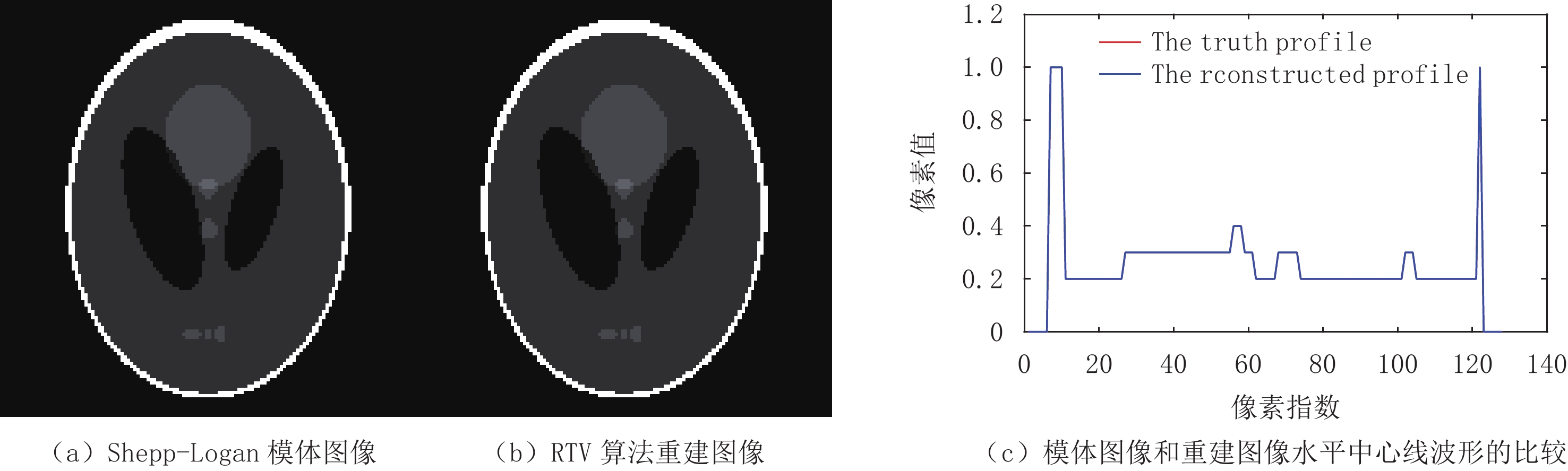
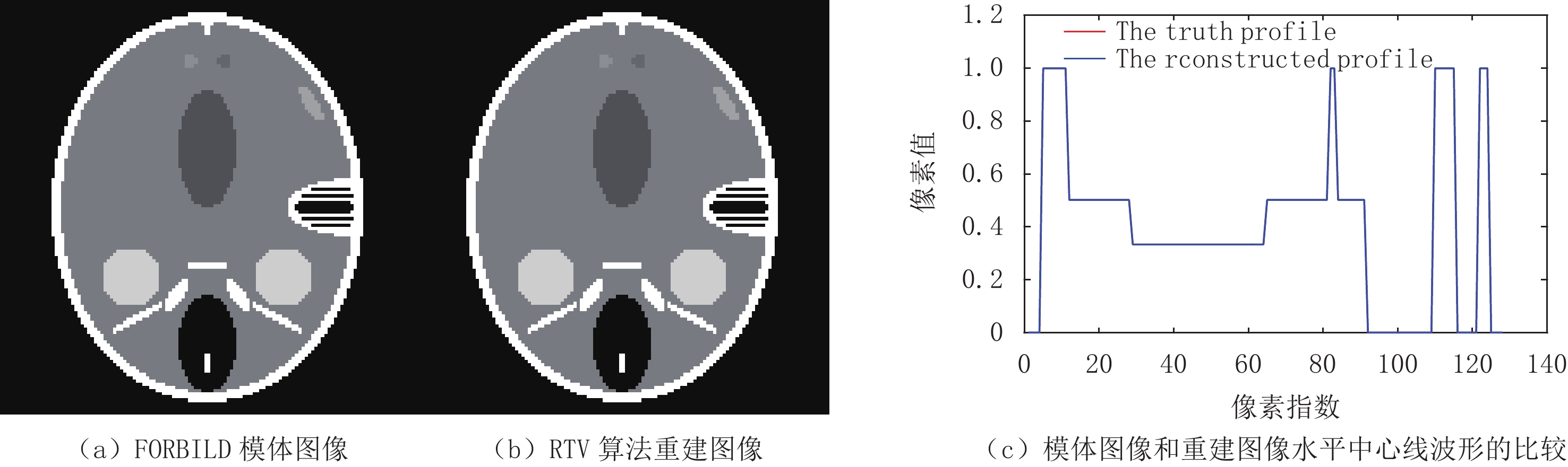
${{\boldsymbol{f}}_{{\rm{res}}}}$ 是重建图像的向量表示,${{\boldsymbol{f}}_{{\rm{truth}}}}$ 是真实图像的向量表示,N为向量长度。$$ {{\rm{RMSE}}\left( {{{\boldsymbol{f}}_{{\rm{rec}}}},{{\boldsymbol{f}}_{{\rm{truth}}}}} \right) = \frac{{{{\big\| {{{\boldsymbol{f}}_{{\rm{rec}}}} - {{\boldsymbol{f}}_{{\rm{truth}}}}} \big\|}_2}}}{{\sqrt N }}} 。 $$ (17) 对于Shepp-Logan模体和FORBILD模体重建来说,当RTV最小化算法分别迭代到200次和300次左右时,其各自的RMSE已经小于10-4,符合该实验定量分析正确性的标准。而从重建结果来看,如图2和图3所示,其中(a)图是Shepp-Logan和FORBILD仿真模型图像;(b)是实现收敛的重建图像;(c)是(a)、(b)两幅图像中心线波形的比较。从图2和图3可见(a)、(b)两幅图几乎完全一样,难以分辨彼此。从(c)图可见(a)、(b)两幅图的中心线波形几乎完全重合。对重建图像和中心线波形的观察表明,该算法实现了高精度重建,符合该实验定性观察正确性的标准。
![]() 图 2 RTV算法的正确性研究关于Shepp-Logan模体的重建结果Figure 2. Correctness research of RTV algorithm on reconstruction results of Shepp-Logan phantom
图 2 RTV算法的正确性研究关于Shepp-Logan模体的重建结果Figure 2. Correctness research of RTV algorithm on reconstruction results of Shepp-Logan phantom![]() 图 3 RTV算法的正确性研究关于FORBILD模体的重建结果Figure 3. Correctness research of RTV algorithm on reconstruction results of FORBILD phantom
图 3 RTV算法的正确性研究关于FORBILD模体的重建结果Figure 3. Correctness research of RTV algorithm on reconstruction results of FORBILD phantom总的来说,无论是从重建结果的定性观察,还是重建图像的RMSE小于
${10^{ - 4}}$ 来看,都可以说明该实验的正确性研究是成功的,从而说明所构建的模型及代码实现是正确的。3.1.3 RTV最小化重建算法的收敛性评估
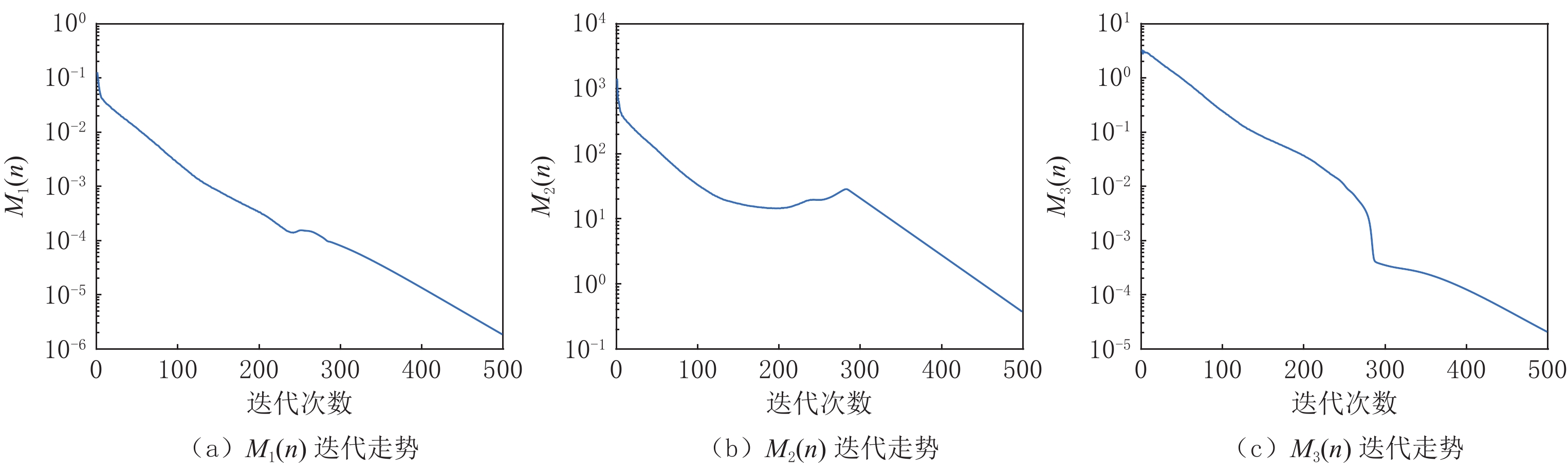
对于算法收敛性的评估,引入以下3个度量标准,通过观察这3个度量标准来判断算法的收敛性:
$$ {{{{M}}_1}\left( n \right) = {\rm{RMSE}}\Big( {{{\boldsymbol{f}}_n},{{\boldsymbol{f}}_{{\rm{truth}}}}} \Big)} \text{,} $$ (18) $$ {{M_2}\left( n \right) = \big\| {{\boldsymbol{g}} - {\boldsymbol{A}}{{\boldsymbol{f}}_n}} \big\|} _2\text{,} $$ (19) $$ {{M_3}\left( n \right) = \frac{{{{\big\| {{{\boldsymbol{f}}_n}} \big\|}_{{\rm{TV}}}} - {{\big\| {{{\boldsymbol{f}}_{{\rm{truth}}}}} \big\|}_{\rm{TV}}}}}{{{{\big\| {{{\boldsymbol{f}}_{{\rm{truth}}}}} \big\|}_{{\rm{TV}}}}}}} \text{,} $$ (20) 其中(18)式代表重建图像与真实图像间的均方根误差;(19)式代表重建图像的投影与真实投影间的差异,(20)式代表重建图像的TV值与真实图像TV值之间的相对误差。
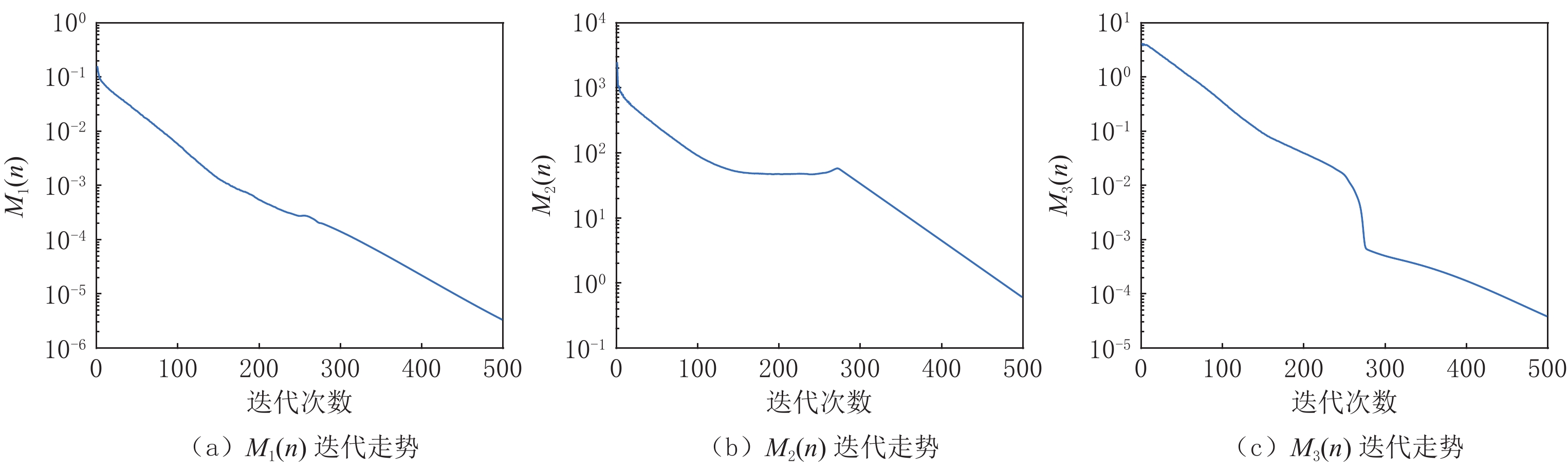
在此实验的研究中,投影数据是充分且准确的,所以在重建图像达到收敛时,这些度量标准要达到充分小,表示该算法在高精度重建的同时达到了收敛。如图4和图5所示,其分别展示了在重建Shepp-Logan和FORBILD模体时RTV最小化重建算法的收敛行为,其中图(a)~图(c)图分别展示了(18)~(20)式所示的度量标准的迭代走势。
![]() 图 4 RTV算法重建Shepp-Logan模体收敛行为的展示Figure 4. Display of convergence behavior when reconstructing Shepp-Logan phantom by RTV algorithm
图 4 RTV算法重建Shepp-Logan模体收敛行为的展示Figure 4. Display of convergence behavior when reconstructing Shepp-Logan phantom by RTV algorithm![]() 图 5 RTV算法重建FORBILD模体收敛行为的展示Figure 5. Display of convergence behavior when reconstructing FORBILD phantom by RTV algorithm
图 5 RTV算法重建FORBILD模体收敛行为的展示Figure 5. Display of convergence behavior when reconstructing FORBILD phantom by RTV algorithm图4和图5中的(a)图显示的是图像误差的迭代走势。而在重建这两个模体时,其
${M_1}\left( n \right)$ 分别迭代到200多次和300多次时达到了10-4,在迭代到500次时分别达到了10-5和10-7,如果继续迭代,其${M_1}\left( n \right)$ 还会有继续下降的趋势;(b)图显示了数据误差的迭代走势,从图中可以看出数据误差在不断减小,但是在重建过程中有一个向上的抖动,这种现象是TV类算法在迭代过程的一个特点,在迭代过程中经常出现,并不会影响该算法的收敛性,振动之后,其相对误差会继续减小,这说明优化模型的解仍然趋向收敛;(c)图显示了TV值的相对误差,从图中可见其整体下降趋势,并且在迭代到500次之后都还有继续下降的趋势。总之,无论是从(a)图,还是(b)图、(c)图来看,重建结果都已在有限次的迭代次数下使误差达到了充分小,并且还有继续下降的趋势,直至达到其收敛态。
3.2 算法稀疏重建能力的评估与正则项各参数的选取
为了评估RTV算法的稀疏重建能力,本节实验分别使用RTV算法和TV算法对FORBILD、Shepp-Logan和真实CT图像模体在20,30,40,50个投影角度下进行模拟实验。这些模体的大小都是128
$ \times $ 128。在实验分析中,使用均方根误差(RMSE)和结构相似性(structural similarity,SSIM)作为图像重建质量的度量。在文献[2]对ASD-POCS算法的阐述中,数据容差
$ \in $ 只强调与噪声强度有关,而本节实验投影数据不含噪声,所以将ε设为 0。对于RTV最小化迭代次数,设定为4,经过大量实验后发现4次迭代已经足够得到相对精确的结果,如果RTV最小化迭代次数偏大的话,重建结果会出现模糊,丢失细节等情况。对于算法的停止条件(stopping criteria),可以设为当达到某个特定条件时结束,如
${{\big\| {{{\boldsymbol{f}}^{(n)}} - {{\boldsymbol{f}}^{(n - 1)}}} \big\|} \mathord{\left/ {\vphantom {{\big\| {{f^{(n)}} - {f^{(n - 1)}}} \big\|} {\big\| {{f^{(n - 1)}}} \big\|}}} \right. } {\big\| {{{\boldsymbol{f}}^{(n - 1)}}} \big\|}} \leq {10^{ - 4}}$ 时结束迭代。但是为了更直观地分析算法迭代过程中RMSE曲线的收敛特性,在本节实验里,将算法的停止条件设为迭代500次后,结束循环。对于RTV正则项的权重参数λ,它影响着算法在保留更多原始投影数据内容和去除噪声之间的平衡。如果λ过大,会增加正则项的权重,这样的话,会导致重建算法在去除更多噪声信息的同时,也会平滑模糊掉重建图像的更多细节;相反,如果λ较小的话,数据保真项的权重会增加,重建图像可能将会过拟合给定的投影数据,相应的数据中的噪声也会被更多地保留。所以,合适的选择是在去噪和保留重建图像细节之间找到一个使两者实现平衡的数值,通过大量实验所得到的经验来看,选择λ=0.45,可以在很好地抑制伪影的同时有效地保护图像结构和细节。
对于参数ε,其在原RTV模型中的作用主要用于避免分母为0的情况出现。在本文算法里,ε有两个作用,一个是避免分母为0的情况出现,另一个是在某种程度上保护图像结构。ε取较小值时,
$ {1 \mathord{\left/ {\vphantom {1 {\left( {{\mathcal{L}_x}\left( {{f_p}} \right) + \varepsilon } \right)}}} \right. } {\left( {{\mathcal{L}_x}\left( {{f_p}} \right) + \varepsilon } \right)}} $ 和$ {1 \mathord{\left/ {\vphantom {1 {\left( {{\mathcal{L}_y}\left( {{f_p}} \right) + \varepsilon } \right)}}} \right. } {\left( {{\mathcal{L}_y}\left( {{f_p}} \right) + \varepsilon } \right)}} $ 会让一部分图像结构的梯度遭受一定程度的惩罚,使得图像结构边界质量退化;ε取较大值时,惩罚减轻,有利于保护图像结构。总的来说,尽管误差不能被完全消除,但取较大的ε有利于提高重建图像的质量,这里取ε=0.025。至于控制WIV和WTV矩形区域空间比例的σ参数,经过大量实验,当σ取 0.25时,可以得到较为精确的实验结果。
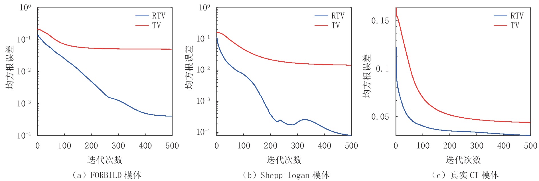
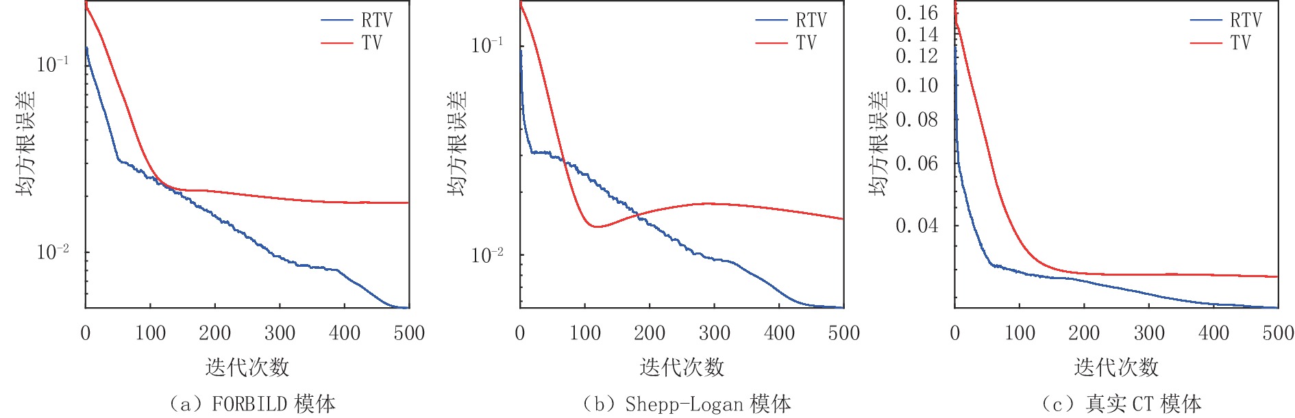
图6中的(a)图显示了FORBILD模体在20个投影角度下使用RTV和TV最小化重建算法的RMSE趋势曲线的比较,显然,RTV最小化重建算法经过500次迭代达到收敛点后拥有更高的重建精度,其最终的收敛精度是30×10-5。而TV算法最终的收敛精度只有5130×10-5。
![]() 图 6 不同模体在20个投影角度下使用RTV和TV最小化重建算法的RMSE趋势曲线的比较Figure 6. Comparison of RMSE trend curves of the same phantom using RTV and TV minimization reconstruction algorithms at 20 projection angles
图 6 不同模体在20个投影角度下使用RTV和TV最小化重建算法的RMSE趋势曲线的比较Figure 6. Comparison of RMSE trend curves of the same phantom using RTV and TV minimization reconstruction algorithms at 20 projection angles表1比较了使用RTV算法化和TV算法在20到50个投影角度下重建FORBILD模体的均方根误差(RMSE)和结构相似性(SSIM)的比较,可见RTV算法的重建图像比TV算法的重建图像有更高的重建精度和结构相似性。
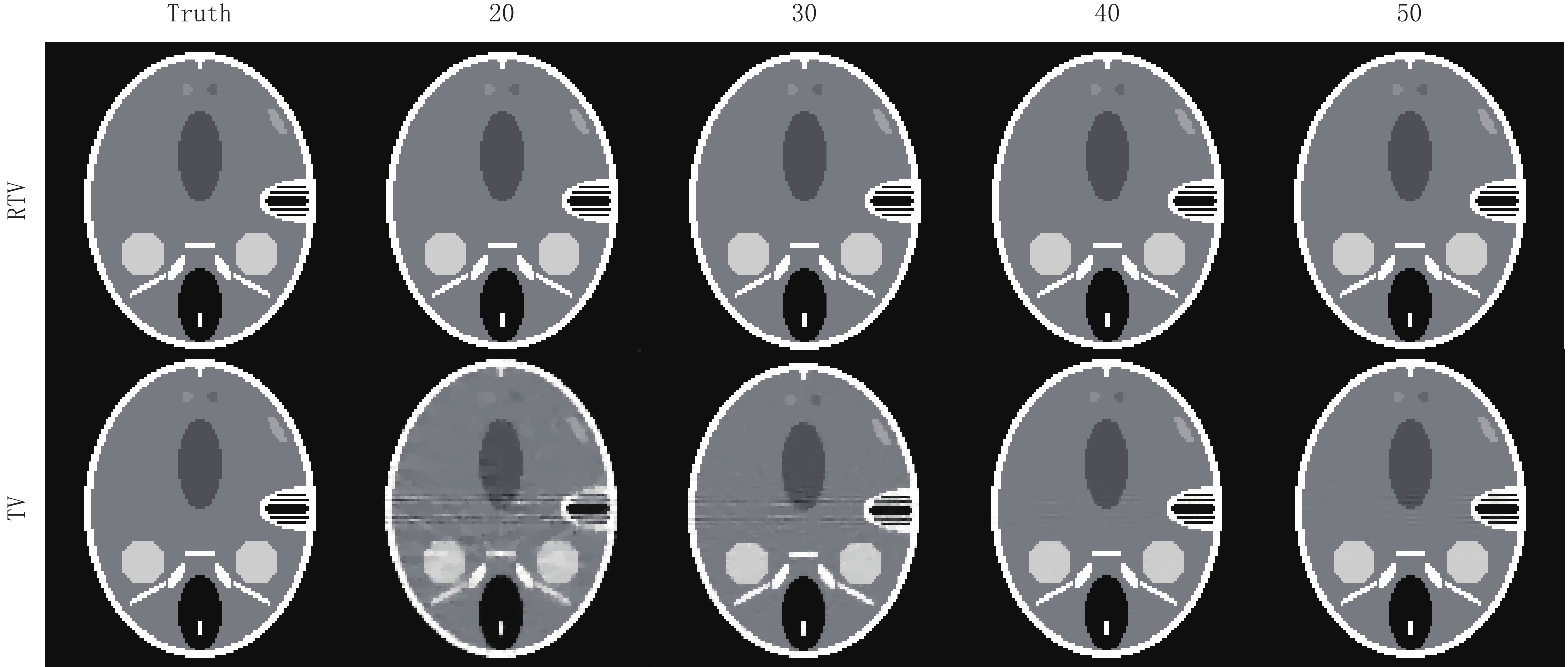
表 1 RTV算法和TV算法重建FORBILD模体的RMSE和SSIM比较Table 1. RMSE and SSIM comparison of RTV and TV algorithms for FORBILD phantom reconstruction项目 算法 投影个数 20 30 40 50 RMSE RTV 30.0×10⁻⁵ 9.96×10⁻⁵ 7.11×10⁻⁵ 5.60×10⁻⁵ TV 5130×10-5 2530×10-5 620×10-5 590×10-5 SSIM RTV 0.9587 0.9792 0.9972 0.9992 TV 0.9293 0.9583 0.9943 0.9986 图7显示了两种算法关于FORBILD模体的重建结果。在20个投影角度下,TV算法重建结果有明显的伪影和噪点,并且有多处图像细节也被平滑掉。从20个到50个投影角度,其重建图像的精度虽然不断升高,不过一直到50个投影角度时,其重建图像与原图相比还是有些明显的伪影。而同样在20个投影角度的情况下,RTV最小化算法重建结果用肉眼几乎看不出与原图的区别。随着投影角度的增加,其重建结果与原图相比还是一致的。显然RTV算法的重建效果更好一点。
![]() 图 7 RTV算法和TV算法对于FORBILD模体重建结果的比较:图像上方的数字表示投影个数;左边文字表示使用的算法Figure 7. Comparison of FORBILD phantom reconstruction results between the RTV algorithm and the TV algorithm: the number above the image represents the number of projections; the text on the left indicates the algorithm used
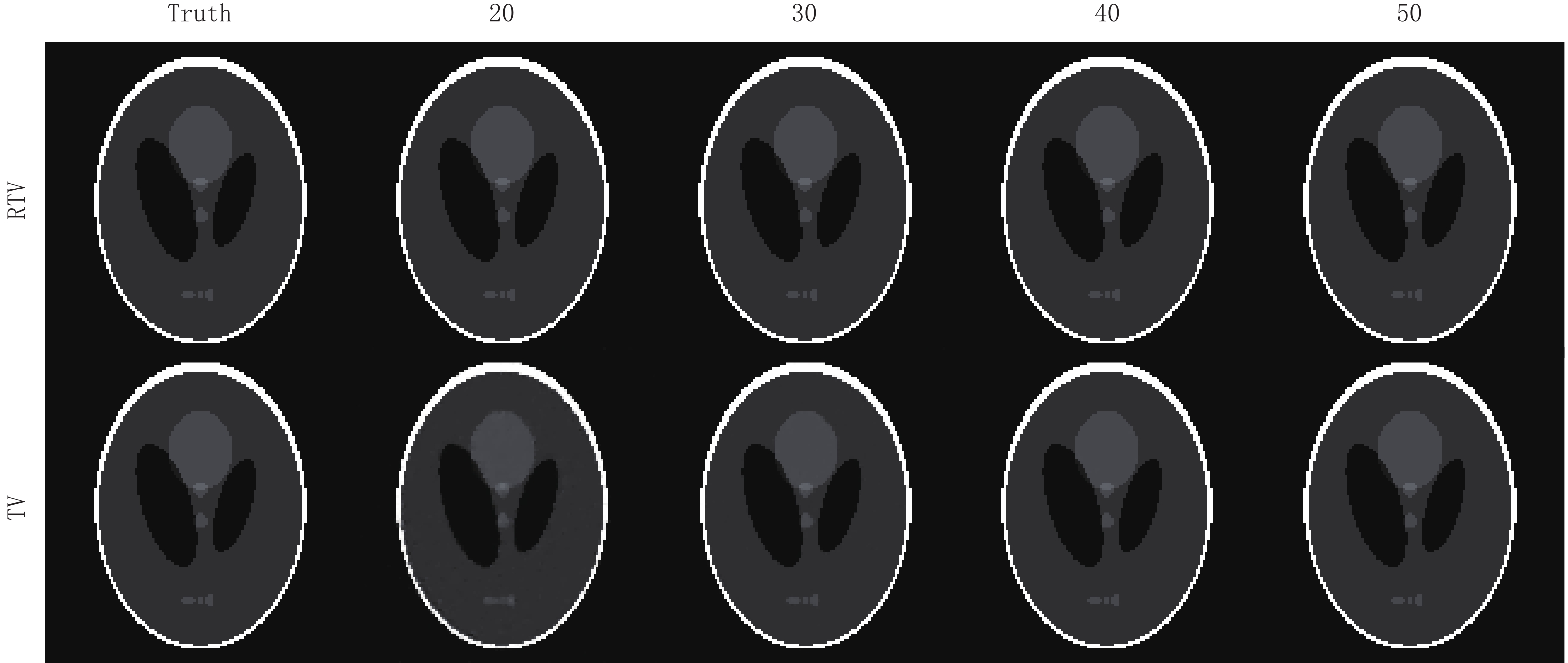
图 7 RTV算法和TV算法对于FORBILD模体重建结果的比较:图像上方的数字表示投影个数;左边文字表示使用的算法Figure 7. Comparison of FORBILD phantom reconstruction results between the RTV algorithm and the TV algorithm: the number above the image represents the number of projections; the text on the left indicates the algorithm used图8显示了两种算法关于Shepp-Logan模体的重建结果,通过对比,可见在20个投影角度下,RTV最小化重建算法的重建结果与原图相比用肉眼几乎看不出与原图的区别。而TV最小化算法在20个投影角度下的重建结果对于图像结构的保护还是有所欠缺,模糊了较多的细节。但随着投影角度的增加,其重建精度也越来越高,两种算法的重建结果与原图相比都几乎一样。
![]() 图 8 RTV算法和TV算法对于Shepp-Logan模体重建结果的比较:图像上方的数字表示投影个数;左边文字表示使用的算法Figure 8. Comparison of Shepp-Logan phantom reconstruction results between the RTV algorithm and the TV algorithm: the number above the image represents the number of projections; the text on the left indicates the algorithm used
图 8 RTV算法和TV算法对于Shepp-Logan模体重建结果的比较:图像上方的数字表示投影个数;左边文字表示使用的算法Figure 8. Comparison of Shepp-Logan phantom reconstruction results between the RTV algorithm and the TV algorithm: the number above the image represents the number of projections; the text on the left indicates the algorithm used图6中的(b)图显示了Shepp-Logan模体在20个投影角度下使用RTV和TV最小化重建算法的RMSE趋势曲线的比较,显然,RTV最小化重建算法经过500次迭代达到收敛点后拥有更高的重建精度,其最终的收敛精度是8.010×10⁻⁵。而TV算法最终的收敛精度只有1610×10-5。
表2比较了使用RTV算法和TV最小化算法在20到50个投影角度下重建Shepp-Logan模体的RMSE和SSIM的比较,可见在Shepp-Logan模体上的重建,RTV最小化重建算法同样具有更高的的重建精度和结构相似性。
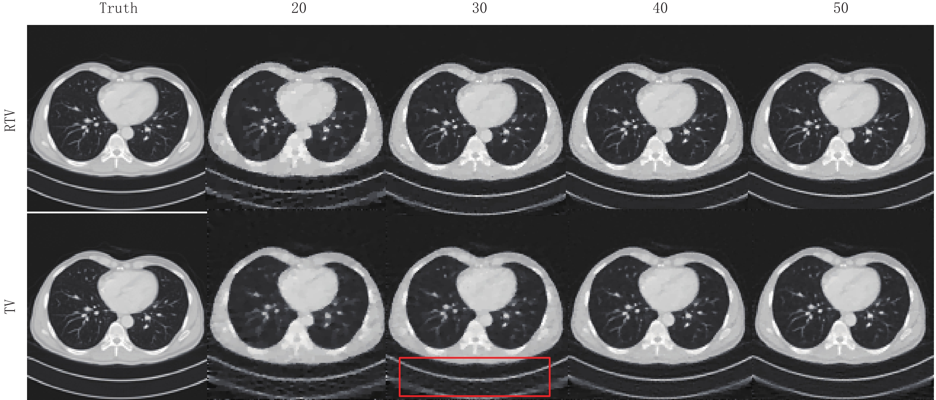
表 2 RTV算法和TV算法重建Shepp-Logan模体的RMSE和SSIM比较Table 2. RMSE and SSIM comparison of the RTV and TV algorithms for Shepp-Logan phantom reconstruction项目 算法 投影个数 20 30 40 50 RMSE RTV 8.010×10⁻⁵ 4.791×10⁻⁵ 3.349×10⁻⁵ 2.586×10⁻⁵ TV 1610×10-5 530×10-5 160×10-5 80×10-5 SSIM RTV 0.9866 0.9948 0.9978 0.9995 TV 0.9812 0.9923 0.9956 0.9991 图9显示了两种算法关于真实CT图像模体的重建图像。在20、30个投影角度下,TV算法明显平滑掉了更多地图像细节,尤其在30个角度下的实验结果里,相比与RTV最小化算法,其重建结果的下面明显有更多伪影。显然,使用RTV最小化算法可以更好地保护图像结构。
![]() 图 9 RTV算法和TV算法对于真实CT图像重建结果的比较:图像上方的数字表示投影个数;左边文字表示使用的算法Figure 9. Comparison of CT-phantom reconstruction results between RTV algorithm and TV algorithm: the number above the image represents the number of projections; The text on the left indicates the algorithm used
图 9 RTV算法和TV算法对于真实CT图像重建结果的比较:图像上方的数字表示投影个数;左边文字表示使用的算法Figure 9. Comparison of CT-phantom reconstruction results between RTV algorithm and TV algorithm: the number above the image represents the number of projections; The text on the left indicates the algorithm used图6中的图(c)显示了真实CT模体图像在20个投影角度下使用RTV和TV最小化重建算法的RMSE趋势曲线的比较,显然,RTV最小化重建算法经过500次迭代达到收敛点后拥有更高的重建精度,其最终的收敛精度是0.0403。而TV算法最终的收敛精度只有0.0467。
表3比较了使用RTV算法化和TV算法在不同投影角度下重建CT真实图像模体的RMSE和SSIM的比较,可以看出,RTV算法比TV算法在CT真实模体上的重建也有更高的重建精度和结构相似性。
表 3 RTV算法和TV算法重建真实CT模体的RMSE和SSIM比较Table 3. RMSE and SSIM comparison of the RTV and TV algorithms for CT phantom reconstruction项目 算法 投影个数 20 30 40 50 RMSE RTV 0.0403 0.0294 0.0210 0.0120 TV 0.0467 0.0302 0.0218 0.0168 SSIM RTV 0.9213 0.9546 0.9743 0.9956 TV 0.8977 0.9387 0.9542 0.9842 3.3 算法去噪能力的评估
为了评估RTV算法的去噪能力,本节实验分别使用RTV最小算法和TV算法对FORBILD、Shepp-Logan和真实CT图像模体在50个投影角度、并分别将不同级别噪声添加到每个投影数据中的情况下进行模拟实验。其中,模体的大小是128×128,高斯噪声的平均值是0,方差分别是0.01、0.02、0.03、0.04、0.05。在实验分析中,使用RMSE和SSIM作为图像重建质量的度量。
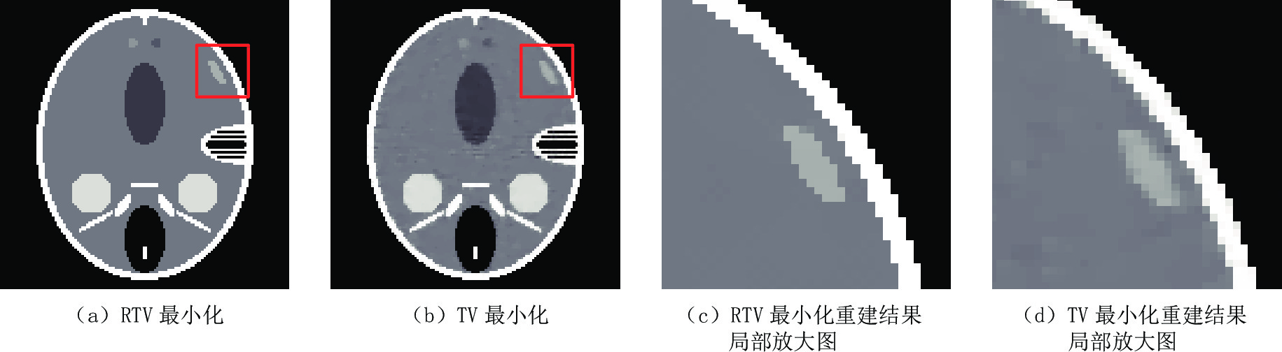
选择FORBILD模体在50个投影角度,并于投影数据中加入方差为0.05的高斯白噪声条件下的重建结果进行阐述。如图10所示,图10(a)是RTV算法的重建结果,图10(b)是TV最小化重建结果,图10(c)和图10(d)分为各自重建结果的局部区域放大图。可见,TV模型和RTV最小化重建模型都显示出了对噪声的抑制特性。但是,通过对比可见,RTV最小化模型重建结果的图像结构明显有着更清晰的边缘间隔,并且从整体看,RTV最小化模型的重建结果更加锐利清晰。
![]() 图 10 在50个投影角度并于投影数据中加入方差为0.05的高斯白噪声条件下分别使用RTV和TV重建算法进行重建的实验结果Figure 10. Under the condition of 50 projection angles and adding Gaussian white noise with a variance of 0.05 to the projection data, RTV and TV minimization reconstruction algorithms are used to reconstruct the results, respectively
图 10 在50个投影角度并于投影数据中加入方差为0.05的高斯白噪声条件下分别使用RTV和TV重建算法进行重建的实验结果Figure 10. Under the condition of 50 projection angles and adding Gaussian white noise with a variance of 0.05 to the projection data, RTV and TV minimization reconstruction algorithms are used to reconstruct the results, respectively图11显示了FORBILD、Shepp-Logan和真实CT模体图像在50个投影角度,并于投影数据中加入方差为0.05的高斯白噪声条件下分别使用RTV和TV最小化重建算法进行重建的RMSE趋势曲线的比较,从表4~表6中的数据可见这两种算法在3个模体上的重建精度分别为0.005和0.01842、0.0055和0.0148、0.0233和0.0286,从定量分析来看显然RTV最小化算法抑制噪声,保护图像结构的效果更好一点。
表 5 RTV算法和TV算法在不同等级噪声下重建Shepp-Logan模体的RMSE和SSIM比较Table 5. Comparison of RMSE and SSM of the RTV and TV algorithms for reconstructing Shepp-Logan phantom under different levels of noise项目 算法 噪声等级 0.01 0.02 0.03 0.04 0.05 RMSE RTV 0.0015 0.0028 0.0035 0.0048 0.0055 TV 0.0065 0.0081 0.0102 0.0126 0.0148 SSIM RTV 0.9943 0.9823 0.9781 0.9653 0.9526 TV 0.9914 0.9814 0.9727 0.9594 0.9512 ![]() 图 11 不同模体在50个投影角度并于投影数据中加入方差为0.05的高斯白噪声条件下使用RTV和TV最小化重建算法重建结果的RMSE趋势曲线的比较Figure 11. Comparison of RMSE trend curves of different phantom reconstruction results the using RTV and TV minimization reconstruction algorithms with 50 projection angles and adding Gaussian white noise with variance of 0.05 added to the projection data表 4 RTV算法和TV算法在不同等级噪声下重建FORBILD模体的RMSE和SSIM比较Table 4. Comparison of RMSE and SSM of the RTV and TV algorithms for reconstructing FORBILD phantom under different levels of noise
图 11 不同模体在50个投影角度并于投影数据中加入方差为0.05的高斯白噪声条件下使用RTV和TV最小化重建算法重建结果的RMSE趋势曲线的比较Figure 11. Comparison of RMSE trend curves of different phantom reconstruction results the using RTV and TV minimization reconstruction algorithms with 50 projection angles and adding Gaussian white noise with variance of 0.05 added to the projection data表 4 RTV算法和TV算法在不同等级噪声下重建FORBILD模体的RMSE和SSIM比较Table 4. Comparison of RMSE and SSM of the RTV and TV algorithms for reconstructing FORBILD phantom under different levels of noise项目 算法 噪声等级 0.01 0.02 0.03 0.04 0.05 RMSE RTV 0.0021 0.0029 0.0032 0.0043 0.0050 TV 0.0085 0.0107 0.0134 0.0162 0.0184 SSIM RTV 0.9923 0.9843 0.9812 0.9756 0.9712 TV 0.9836 0.9793 0.9754 0.9698 0.9652 表 6 RTV算法和TV算法在不同等级噪声下重建真实CT模体的RMSE和SSIM比较Table 6. Comparison of RMSE and SSM of the RTV and TV algorithms for reconstructing CT phantom under different levels of noise项目 算法 噪声等级 0.01 0.02 0.03 0.04 0.05 RMSE RTV 0.0188 0.0198 0.0205 0.0225 0.0233 TV 0.0194 0.0215 0.0233 0.0247 0.0286 SSIM RTV 0.9258 0.9042 0.8938 0.8814 0.8715 TV 0.9123 0.8926 0.8626 0.8612 0.8523 3.4 正则项参数
$\lambda $ 和$\varepsilon $ 的选取对重建结果的影响在本节实验中,并不计划得到使重建结果最优的参数组合,仅通过选取不同的参数值,在其他条件一致的情况下,讨论不同参数值对重建结果的影响。
3.4.1 参数
$\lambda $ 的选取对重建结果的影响在RTV正则项中,参数λ被用来控制正则项的强度,所以选择合适的λ对于CT重建非常重要。在本节实验里,为了排除其他因素的影响,使用无噪声的投影数据,并固定其他的重建参数进行重建。
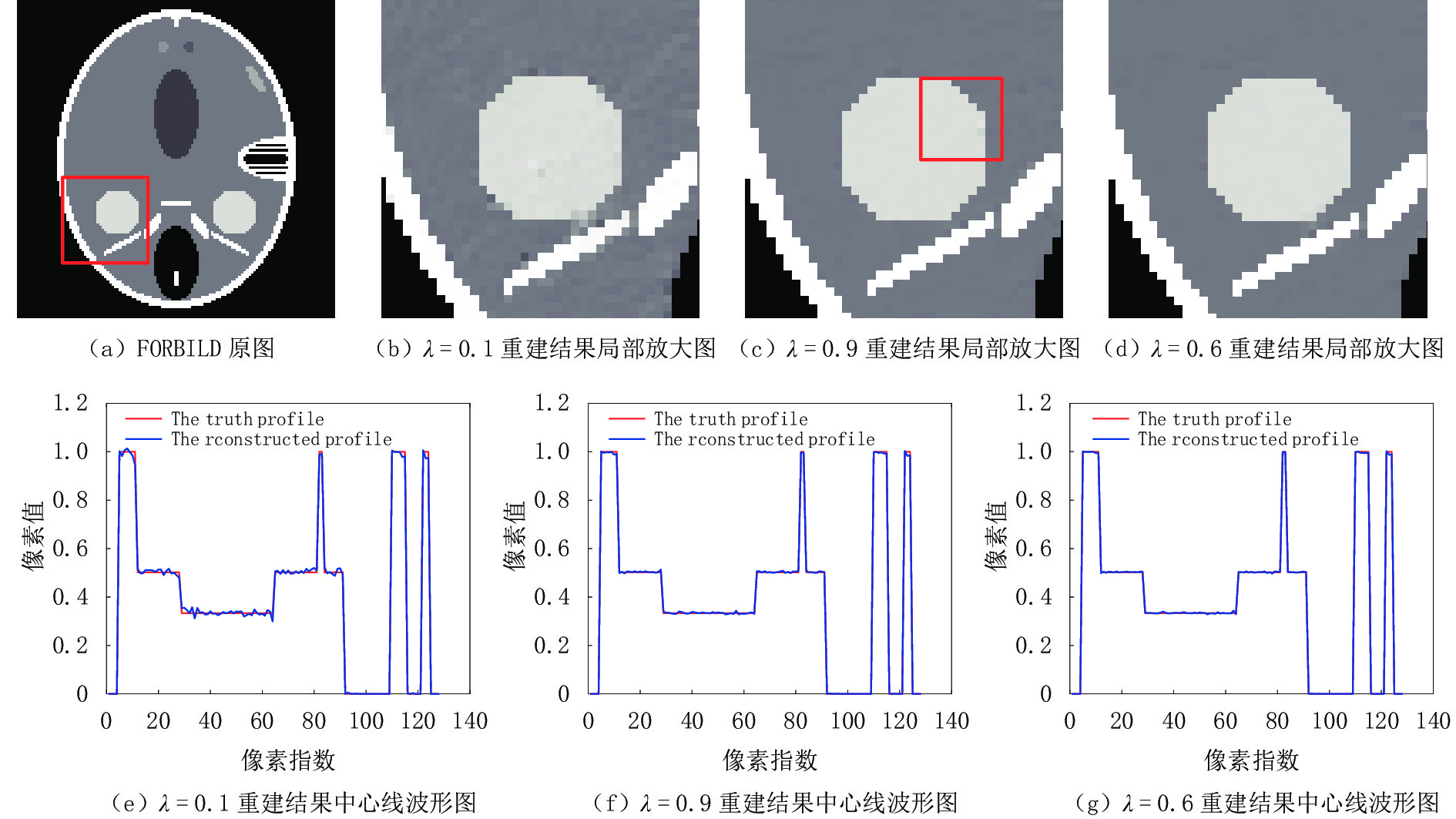
为了探索参数λ不同数值的选取对重建结果的影响,本节实验从0.01到1之间选取了20个不同的数值,然后选择0.1、0.6和0.9三个代表性结果做出讨论。
实验结果如图12所示,图12(a)是原图,图12(b)~图12(d)分别是λ选取不同数值重建结果的局部放大图。图12(e)~图12(g)分别是不同数值重建结果各自所对应的中心线波形图。如图12(c)所示,当λ取0.9时,与图b相比较大的λ可以增加RTV正则项的权重,在有效保护图像结构的同时还可以明显的减少伪影。然而,与图12(d)相比,过大的λ又会使重建图像丢失一些细节。从图12(g)图中可见,当λ=0.6时,其重建图像的中心线波形图与原图的几乎完全重合。所以如果选择合适的λ,在有效抑制伪影的同时还可以很好的保护图像结构。
![]() 图 12 λ不同取值的实验结果和其各自对应的中心线波形图Figure 12. Experimental results with different λ values and their corresponding centerline waveforms
图 12 λ不同取值的实验结果和其各自对应的中心线波形图Figure 12. Experimental results with different λ values and their corresponding centerline waveforms3.4.2 参数ε的选取对重建结果的影响
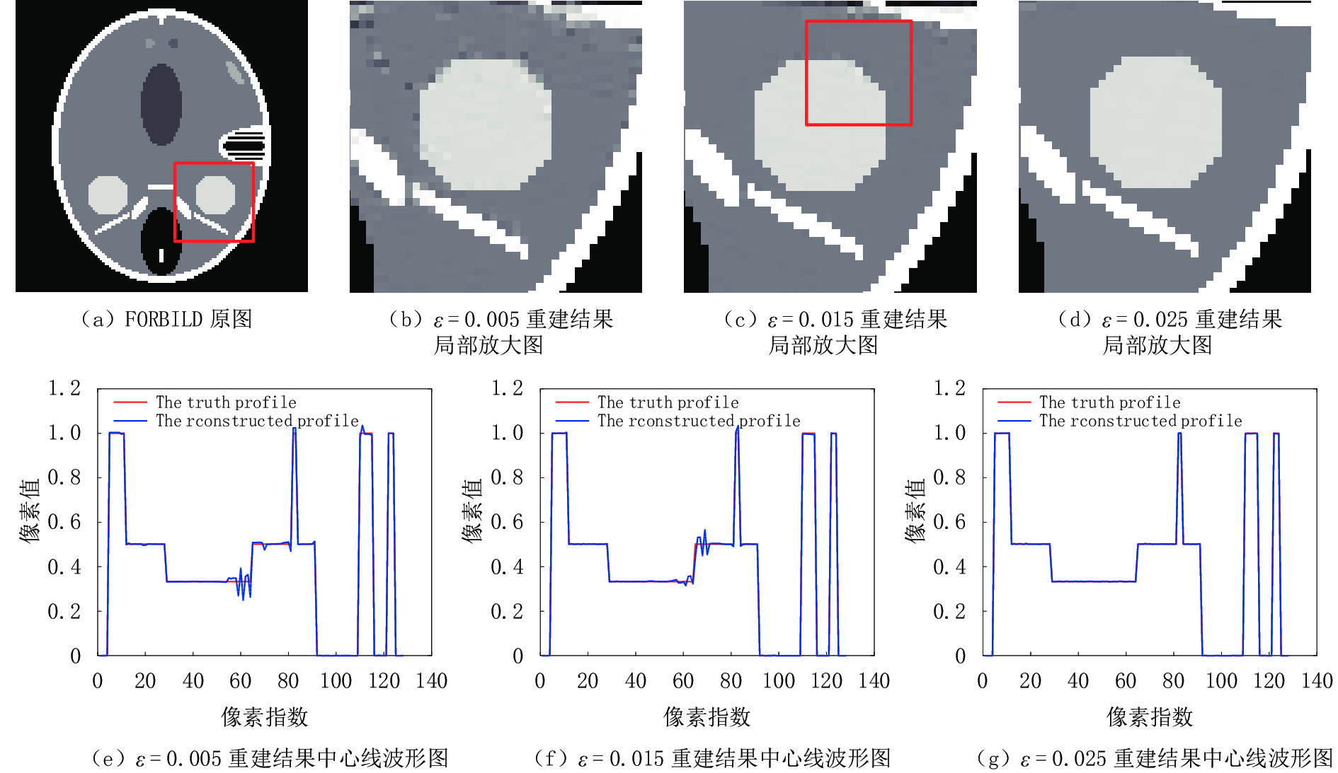
在RTV正则项中,参数ε一是为了避免分母为 0的情况出现,二是在一定程度上可以保护图像结构。这里仍然使用无噪声的投影数据,固定其他重建参数,探索参数ε不同数值的选取对重建结果的影响。选择3个典型的ε值的重建结果进行阐述:0.005、0.015和0.025。
如图13所示,(a)是原图,图13(b)~图13(d)是ε取不同数值的实验结果局部区域放大图,图13(e)~图13(g)是其各自对应的中心线波形图。如图13(b)所示,当ε取较小值时,由于
${1/ {\Big( {{\mathcal{L}_x}\left( {{{\boldsymbol{f}}_p}} \right) + \varepsilon } \Big)}}$ 和${1/ {\Big( {{\mathcal{L}_y}\left( {{{\boldsymbol{f}}_p}} \right) + \varepsilon } \Big)}}$ 会让一部分图像结构的梯度遭受一定程度的惩罚,从而使图像结构边界质量退化,平滑模糊掉重建结果的更多细节;当ε取较大值时,重建结果如图d所示,惩罚相对减轻,有利于保护图像结构。并且通过图12(e)~图12(g)图的对比,我们发现,当ε=0.025取较大值时,其重建结果的中心线波形图与原图更一致。总的来说,尽管误差不能被完全消除,但取较大的ε有利于提高重建图像的质量。![]() 图 13 ε不同取值的实验结果和其各自对应的中心线波形图Figure 13. Experimental results with different ε values and their corresponding centerline waveforms
图 13 ε不同取值的实验结果和其各自对应的中心线波形图Figure 13. Experimental results with different ε values and their corresponding centerline waveforms4. 结论
本文提出了一种基于相对TV最小的CT图像重建模型,通过实验确定了重建模型中的大部分参数,并且设计在ASD-POCS框架下相应的求解算法。该重建模型在保护有效结构的同时在一定程度上提高了重建精度。在CT图像稀疏重建中,TV算法会对重建图像中的所有梯度施加惩罚,而RTV重建模型可以准确地区分图像中的结构和噪声从而施加不同的惩罚,并借此在RTV最小化的过程更准确地缩小模拟投影与真实投影间的差距,以此来保护图像的有效结构并抑制噪声。
本文的研究目的是探索RTV作为正则项被应用于CT重建中的性能及可能的重建优势。实验结果表明,RTV最小化重建算法可以取得比TV最小化算法更高的重建精度。本文所使用的求解算法框架是ASD-POCS框架,需要经过大量的实验得到合适的重建参数,如何避免参数的人为设定,这将是本文下一步的研究内容之一。
-
![]()
图 2 RTV算法的正确性研究关于Shepp-Logan模体的重建结果
Figure 2. Correctness research of RTV algorithm on reconstruction results of Shepp-Logan phantom
![]()
图 3 RTV算法的正确性研究关于FORBILD模体的重建结果
Figure 3. Correctness research of RTV algorithm on reconstruction results of FORBILD phantom
![]()
图 4 RTV算法重建Shepp-Logan模体收敛行为的展示
Figure 4. Display of convergence behavior when reconstructing Shepp-Logan phantom by RTV algorithm
![]()
图 5 RTV算法重建FORBILD模体收敛行为的展示
Figure 5. Display of convergence behavior when reconstructing FORBILD phantom by RTV algorithm
![]()
图 6 不同模体在20个投影角度下使用RTV和TV最小化重建算法的RMSE趋势曲线的比较
Figure 6. Comparison of RMSE trend curves of the same phantom using RTV and TV minimization reconstruction algorithms at 20 projection angles
![]()
图 7 RTV算法和TV算法对于FORBILD模体重建结果的比较:图像上方的数字表示投影个数;左边文字表示使用的算法
Figure 7. Comparison of FORBILD phantom reconstruction results between the RTV algorithm and the TV algorithm: the number above the image represents the number of projections; the text on the left indicates the algorithm used
![]()
图 8 RTV算法和TV算法对于Shepp-Logan模体重建结果的比较:图像上方的数字表示投影个数;左边文字表示使用的算法
Figure 8. Comparison of Shepp-Logan phantom reconstruction results between the RTV algorithm and the TV algorithm: the number above the image represents the number of projections; the text on the left indicates the algorithm used
![]()
图 9 RTV算法和TV算法对于真实CT图像重建结果的比较:图像上方的数字表示投影个数;左边文字表示使用的算法
Figure 9. Comparison of CT-phantom reconstruction results between RTV algorithm and TV algorithm: the number above the image represents the number of projections; The text on the left indicates the algorithm used
![]()
图 10 在50个投影角度并于投影数据中加入方差为0.05的高斯白噪声条件下分别使用RTV和TV重建算法进行重建的实验结果
Figure 10. Under the condition of 50 projection angles and adding Gaussian white noise with a variance of 0.05 to the projection data, RTV and TV minimization reconstruction algorithms are used to reconstruct the results, respectively
![]()
图 11 不同模体在50个投影角度并于投影数据中加入方差为0.05的高斯白噪声条件下使用RTV和TV最小化重建算法重建结果的RMSE趋势曲线的比较
Figure 11. Comparison of RMSE trend curves of different phantom reconstruction results the using RTV and TV minimization reconstruction algorithms with 50 projection angles and adding Gaussian white noise with variance of 0.05 added to the projection data
![]()
图 12 λ不同取值的实验结果和其各自对应的中心线波形图
Figure 12. Experimental results with different λ values and their corresponding centerline waveforms
![]()
图 13 ε不同取值的实验结果和其各自对应的中心线波形图
Figure 13. Experimental results with different ε values and their corresponding centerline waveforms
1. Repeat main loop 13. $for{\text{ } }i = 1{\text{:} }{N_{{\rm{grad}}} }{\text{ do RTV - ASD loop} }$: 2. $ {{\boldsymbol{f}}}_{p}={{\boldsymbol{f}}}^{(n)}$ ${\boldsymbol{d} }{ {\boldsymbol{f} }^{(k)} } = {\nabla _f}\left\| { { {\boldsymbol{f} }^{(n)} } } \right\|_{{\rm{RTV}}}^{(k)}$ 3. ${\text{for } }i = 1{\text{ : } }{N_d}{\text{ do } }{\boldsymbol{f} } = {\boldsymbol{f} } + \beta { {\boldsymbol{A} }_{\boldsymbol{i} } }\displaystyle \frac{ { {g_i} - { {\boldsymbol{A} }_{\boldsymbol{i} } }{\boldsymbol{ \times f} } } }{ { { {\boldsymbol{A} }_{\boldsymbol{i} } }{\boldsymbol{ \times } }{ {\boldsymbol{A} }_{\boldsymbol{j} } } } }$ $ {\boldsymbol{d}}{{\boldsymbol{f}}^{(k)}} = {{{\boldsymbol{d}}{{\boldsymbol{f}}^{(k)}}} \mathord{\left/ {\vphantom {{{\boldsymbol{d}}{{\boldsymbol{f}}^{(k)}}} {{{\left\| {{\boldsymbol{d}}{{\boldsymbol{f}}^{(k)}}} \right\|}_2}}}} \right. } {{{\left\| {{\boldsymbol{d}}{{\boldsymbol{f}}^{(k)}}} \right\|}_2}}} $ 4. ${\text{for } }i = 1{\text{ : } }{N_i}{\text{ do if } }{{\boldsymbol{f}}_i} < 0{\text{ then } }{{\boldsymbol{f}}_i} = 0$ $ {{\boldsymbol{f}}^{(n)}} = {{\boldsymbol{f}}^{(n)}} - {d_\alpha }*{\boldsymbol{d}}{{\boldsymbol{f}}^{(k)}} $ 5. ${ {\boldsymbol{f} }_{{\rm{res}}} } = { {\boldsymbol{f} }^{(n)} }$ end for 6. ${{\boldsymbol{g}}^{(n)}} = {\boldsymbol{A}} \times {{\boldsymbol{f}}^{(n)}}$ 14. $ \nabla {{\boldsymbol{f}}_{{\text{RTV}}}} = {\left\| {{{\boldsymbol{f}}^{(n)}} - {{\boldsymbol{f}}_p}} \right\|_2} $ 7. ${d_p} = {\left\| {{{\boldsymbol{g}}^{(n)}}{\boldsymbol{ - }}{{\boldsymbol{g}}_{\boldsymbol{0}}}} \right\|_2}$ 15. ${\rm{if}}{\text{ } }\nabla { {\boldsymbol{f} }_{ {\text{RTV} } } } > {r_{\max} }*\nabla { {\boldsymbol{f} }_{ {\text{POCX} } } }{\text{ } }{\rm{and}}{\text{ } }{d_p} > \in {\text{ then} }$ 10. $\nabla {{\boldsymbol{f}}_{{\text{POCX}}}} = {\left\| {{{\boldsymbol{f}}^{(n)}} - {{\boldsymbol{f}}_p}} \right\|_2}$ ${d_\alpha } = {d_\alpha }*{\alpha _{{\rm{red}}} }$ 11. ${\text{if first iterarion , then }}{d_\alpha } = \alpha \cdot \nabla {{\boldsymbol{f}}_{{\text{POCX}}}}$ 16. $\beta = \beta \cdot {\beta _{{\rm{red}}} }$ 12. ${{\boldsymbol{f}}_p} = {{\boldsymbol{f}}^{(n)}}$ 17. ${\text{until}}\left\{ {{\text{stopping criteria}}} \right\}$ 18. ${\text{return } }\;{{\boldsymbol{f}}_{ {\rm{res} } } }$  下载: 导出CSV
表 1 RTV算法和TV算法重建FORBILD模体的RMSE和SSIM比较
Table 1 RMSE and SSIM comparison of RTV and TV algorithms for FORBILD phantom reconstruction
项目 算法 投影个数 20 30 40 50 RMSE RTV 30.0×10⁻⁵ 9.96×10⁻⁵ 7.11×10⁻⁵ 5.60×10⁻⁵ TV 5130×10-5 2530×10-5 620×10-5 590×10-5 SSIM RTV 0.9587 0.9792 0.9972 0.9992 TV 0.9293 0.9583 0.9943 0.9986
下载: 导出CSV
表 2 RTV算法和TV算法重建Shepp-Logan模体的RMSE和SSIM比较
Table 2 RMSE and SSIM comparison of the RTV and TV algorithms for Shepp-Logan phantom reconstruction
项目 算法 投影个数 20 30 40 50 RMSE RTV 8.010×10⁻⁵ 4.791×10⁻⁵ 3.349×10⁻⁵ 2.586×10⁻⁵ TV 1610×10-5 530×10-5 160×10-5 80×10-5 SSIM RTV 0.9866 0.9948 0.9978 0.9995 TV 0.9812 0.9923 0.9956 0.9991
下载: 导出CSV
表 3 RTV算法和TV算法重建真实CT模体的RMSE和SSIM比较
Table 3 RMSE and SSIM comparison of the RTV and TV algorithms for CT phantom reconstruction
项目 算法 投影个数 20 30 40 50 RMSE RTV 0.0403 0.0294 0.0210 0.0120 TV 0.0467 0.0302 0.0218 0.0168 SSIM RTV 0.9213 0.9546 0.9743 0.9956 TV 0.8977 0.9387 0.9542 0.9842
下载: 导出CSV
表 5 RTV算法和TV算法在不同等级噪声下重建Shepp-Logan模体的RMSE和SSIM比较
Table 5 Comparison of RMSE and SSM of the RTV and TV algorithms for reconstructing Shepp-Logan phantom under different levels of noise
项目 算法 噪声等级 0.01 0.02 0.03 0.04 0.05 RMSE RTV 0.0015 0.0028 0.0035 0.0048 0.0055 TV 0.0065 0.0081 0.0102 0.0126 0.0148 SSIM RTV 0.9943 0.9823 0.9781 0.9653 0.9526 TV 0.9914 0.9814 0.9727 0.9594 0.9512
下载: 导出CSV
表 4 RTV算法和TV算法在不同等级噪声下重建FORBILD模体的RMSE和SSIM比较
Table 4 Comparison of RMSE and SSM of the RTV and TV algorithms for reconstructing FORBILD phantom under different levels of noise
项目 算法 噪声等级 0.01 0.02 0.03 0.04 0.05 RMSE RTV 0.0021 0.0029 0.0032 0.0043 0.0050 TV 0.0085 0.0107 0.0134 0.0162 0.0184 SSIM RTV 0.9923 0.9843 0.9812 0.9756 0.9712 TV 0.9836 0.9793 0.9754 0.9698 0.9652
下载: 导出CSV
表 6 RTV算法和TV算法在不同等级噪声下重建真实CT模体的RMSE和SSIM比较
Table 6 Comparison of RMSE and SSM of the RTV and TV algorithms for reconstructing CT phantom under different levels of noise
项目 算法 噪声等级 0.01 0.02 0.03 0.04 0.05 RMSE RTV 0.0188 0.0198 0.0205 0.0225 0.0233 TV 0.0194 0.0215 0.0233 0.0247 0.0286 SSIM RTV 0.9258 0.9042 0.8938 0.8814 0.8715 TV 0.9123 0.8926 0.8626 0.8612 0.8523
下载: 导出CSV
-
[1] PAN X, SIDKY E Y, VANNIER M. Why do commercial CT scanners still employ traditional, filtered back-projection for image reconstruction?[J]. Inverse Problems, 2008, 25(12): 1230009.
[2] SIDKY E Y, PAN X. Image reconstruction in circular cone-beam computed tomography by constrained, total-variation minimization[J]. Physics in Medicine & Biology, 2008, 53(17): 4777−4807.
[3] YU L, YU Z, SIDKY E Y, et al. Region of interest reconstruction from truncated data in circular cone-beam CT[J]. IEEE Transactions on Medical Imaging, 2006, 25(7): 869−881. doi: 10.1109/TMI.2006.872329
[4] CANDES E, ROMBERG J, TAO T. Robust uncertainty principles: Exact signal reconstruction from highly incomplete frequency information[J]. IEEE Transactions on Information Theory, 2006, 52(2): 489-509.
[5] VOGEL C R. Iterative method for total variation denoising[J]. SIAM Journal on Scientific Computing, 1996, 17(1): 227−238. doi: 10.1137/0917016
[6] SIDKY E Y, EMIL Y, KAO C M, et al. Accurate image reconstruction from few-views and limited-angle data in divergent-beam CT[J]. Journal of X-ray Science & Technology, 2006, 14: 119−139.
[7] DONOHO D L. Compressed sensing[J]. IEEE Transactions on Information Theory, 2006, 52: 1289-1306.
[8] LIU B, KATSEVICH A, YU H. Interior tomography with curvelet-based regularization[J]. Journal of X-ray Science and Technology, 2016, 25(1): 1−13.
[9] SIDKY E Y, CHARTRAND R, BOONE J M, et al. Constrained TpV minimization for enhanced exploitation of gradient sparsity: Application to CT image reconstruction[J]. IEEE Journal of Translational Engineering in Health & Medicine, 2014, 2(6): 1−18.
[10] CHAMBOLLE A, POCK T. An introduction to continuous optimization for imaging[J]. Acta Numerica, 2016, 25: 161-319.
[11] MBOLLE A, POCK T. A first-order primal-dual algorithm for convex problems with applications to imaging[J]. Journal of Mathematical Imaging and Vision, 2011, 40(1): 120−145. doi: 10.1007/s10851-010-0251-1
[12] SIDKY E Y, JRGENSEN J H, PAN X. Convex optimization problem prototyping for image reconstruction in computed tomography with the Chambolle-Pock algorithm[J]. Physics in Medicine & Biology, 2011, 57(10): 3065−3091.
[13] XU L, YAN Q, XIA Y, et al. Structure extraction from texture via relative total variation[J]. ACM Transactions on Graphics, 2012, 31(6): 139.
[14] RIGIE D S, RIVIèRE P L. Joint reconstruction of multi-channel, spectral CT data via constrained total nuclear variation minimization[J]. Physics in Medicine & Biology, 2015, 60(5): 1741.
[15] QIAO Z, REDLER G, EPEL B, et al. A balanced total-variation-Chambolle-Pock algorithm for EPR imaging[J]. Journal of Magnetic Resonance, 2021, 328: 107009. doi: 10.1016/j.jmr.2021.107009
[16] 闫慧文, 乔志伟. 基于ASD-POCS框架的高阶TpV图像重建算法[J]. CT理论与应用研究, 2021,30(3): 279−289. DOI: 10.15953/j.1004-4140.2021.30.03.01. YAN H W, QIAO Z W. High order TPV image reconstruction algorithm based on ASD-POCS framework[J]. CT Theory and Applications, 2021, 30(3): 279−289. DOI: 10.15953/j.1004-4140.2021.30.03.01. (in Chinese).
[17] XIN J, LIANG L, CHEN Z, et al. Anisotropic total variation minimization method for limited-angle CT reconstruction[C]//Proc. SPIE 8506, Developments in X-ray Tomography VIII, 85061C, 2012. https://doi.org/10.1117/12.930339.
[18] YU H, WANG G. A soft-threshold filtering approach for reconstruction from a limited number of projections[J]. Physics in Medicine & Biology, 2010, 55(13): 3905−3916.
[19] 乔志伟. 总变差约束的数据分离最小图像重建模型及其Chambolle-Pock求解算法[J]. 物理学报, 2018,67(19): 198701. DOI: 10.7498/aps.67.20180839. QIAO Z W. Total variation constrained data separation minimum image reconstruction model and its Chambolle-Pock algorithm[J]. Acta Physica Sinica, 2018, 67(19): 198701. DOI: 10.7498/aps.67.20180839. (in Chinese).
[20] YU Z, NOO F, DENNERLEIN F, et al. Simulation tools for two-dimensional experiments in X-ray computed tomography using the FORBILD head phantom[J]. Physics in Medicine & Biology, 2012, 57(13): 237−252.
[21] SIDDON R L. Fast calculation of the exact radiological path for a three-dimensional CT array[J]. Medical Physics, 1985, 12(2): 252−255. doi: 10.1118/1.595715
[22] GORDON R, BENDER R, HERMAN G T. Algebraic reconstruction techniques (ART) for three-dimensional electron microscopy and X-ray photography[J]. Journal of Theoretical Biology, 1970, 29(3): 471−481. doi: 10.1016/0022-5193(70)90109-8
-
期刊类型引用(3)
1. 赵浩翔,赵晓杰,陈平,魏交统. 基于散射校正板和ADMM算法的锥束CT散射校正. CT理论与应用研究(中英文). 2025(02): 225-234 .  百度学术
百度学术
2. 易焜然,王晗,詹道桦,史卓豪,陈艺宾,房飞宇. 基于多方向总变分的稀疏角度CT图像重建算法. 激光与光电子学进展. 2025(06): 49-55 . 百度学术
3. 王红霞,龚长城. 基于ASD-POCS算法框架的自引导图像滤波重建算法. 中国体视学与图像分析. 2024(04): 303-310 . 百度学术
其他类型引用(2)


计量
- 文章访问数: 810
- HTML全文浏览量: 260
- PDF下载量: 174
- 被引次数: 5
目录
1. 相关知识
1.1 成像模型
1.2 TV最小化重建模型
1.3 RTV模型
2. 本文方法
2.1 RTV最小化重建模型
2.2 RTV最小化重建模型求解算法伪代码
3. 实验结果与分析
3.1 算法的正确性和收敛性研究
3.1.1 仿真模体及实验条件
3.1.2 RTV最小化重建算法的正确性研究
3.1.3 RTV最小化重建算法的收敛性评估
3.2 算法稀疏重建能力的评估与正则项各参数的选取
3.3 算法去噪能力的评估
3.4 正则项参数
$\lambda $ 和$\varepsilon $ 的选取对重建结果的影响3.4.1 参数
$\lambda $ 的选取对重建结果的影响3.4.2 参数ε的选取对重建结果的影响
4. 结论