SHEN L, LU Q, TANG H, et al. A feasibility study of knee joint semantic segmentation on 3D MR images[J]. CT Theory and Applications, 2022, 31(5): 531-542. DOI: 10.15953/j.ctta.2022.091.
Citation:
SHEN L, LU Q, TANG H, et al. A feasibility study of knee joint semantic segmentation on 3D MR images[J]. CT Theory and Applications, 2022, 31(5): 531-542. DOI: 10.15953/j.ctta.2022.091.
SHEN L, LU Q, TANG H, et al. A feasibility study of knee joint semantic segmentation on 3D MR images[J]. CT Theory and Applications, 2022, 31(5): 531-542. DOI: 10.15953/j.ctta.2022.091.
Citation:
SHEN L, LU Q, TANG H, et al. A feasibility study of knee joint semantic segmentation on 3D MR images[J]. CT Theory and Applications, 2022, 31(5): 531-542. DOI: 10.15953/j.ctta.2022.091.
The segmentation of knee joint is of great significance for diagnosis, guidance and treatment of knee osteoarthritis. However, manual delineation is time-consuming and labor-intensive since various anatomical structures are involved in the 3D MRI volume. Automatic segmentation of the whole knee joint requires no human effort, additionally can improve the quality of arthritis diagnosis and treatment by describing the details more accurately. Existing knee joint segmentation methods in the literature focus on only one or few structures out of many. In this paper, we study the feasibility of knee joint segmentation on MR images based on neural networks and deal with the following challenges: (1) end-to-end segmentation of 15 anatomical structures, including bone and soft tissue, of the whole knee on MR images; (2) robust segmentation of small structures such as the anterior cruciate ligament, accounting for about 0.036% of the volume data. Experiments on the knee joint MR images demonstrate that the average segmentation accuracy of our method achieves 92.92%. The Dice similarity coefficients of 9 structures were above 94%, five structures were between 87% and 90%, and the remaining one was about 76%.
Knee osteoarthritis (OA) is one of the most common types of chronic arthritis. The main symptoms are joint pain, stiffness, and restricted mobility, which seriously affect the life quality of patients[1-3]. Among all available clinical diagnostic imaging modalities, MR imaging is the only one that can discriminate soft tissue, cartilage and fluid, providing high-quality images for diagnosing and treating various diseases[4-5]. In general, the injury and inflammation of the keen joint can be imaged more sensitively and accurately by MR imaging. Many previous works have studied the relationship between cartilage degeneration and joint pain[6-7], but more and more studies have shown that other structure lesions can also lead to knee joint pain[8-10]. With the growth of knee MR examinations, the radiologists are overwhelmed. Considering that if the key parts of the knee joints are segmented, the 3D reconstruction results and a more precise region of interest can be provided to the doctors, which can significantly improve the efficiency and quality of radiology workflow.
In recent years, deep learning techniques have attracted attention in the field of medical imaging and have been applied to the segmentation of knee joint MR images. Norman et al. first proposed using a 2D U-Net to automatically segment and classify different subcompartments of the knee at MR images-cartilage and meniscus. It demonstrated that automatic segmentation can increase the speed and accuracy of the diagnosis workflow[11]. In Prasoon et al.[12], a novel tri-planar convolutional neural network was proposed for knee cartilage segmentation. Moreover, it performed better in segmenting tibia cartilage with OA than 3D segmentation methods. Sibaji et al.[13] introduced a conditional generation adversarial model integrating 2D U-Net to improve the segmentation performance. With a modified objective function combining conventional loss and discriminator loss, the average segmentation accuracy of cartilage and meniscus achieved 89%. Zhao et al. proposed a segmentation pipeline combining a 2D encoder-decoder network, 3D fully connected conditional field and 3D simplex deformable model to improve knee joint segmentation efficiency and accuracy[14]. Encoder-decoder network has shown promising results for segmenting cartilage and meniscus. However, few studies focused on the performance of 3D segmentation, and to our best knowledge, no related works involved an end-to-end 3D whole knee joint segmentation.
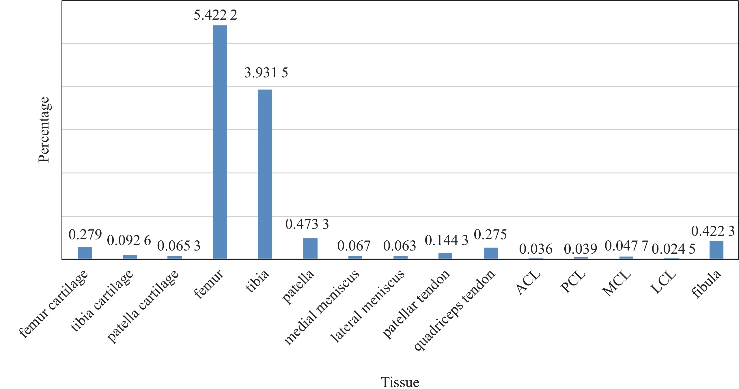
The proportion of different knee anatomical structures varies greatly. There are a total of fifteen anatomical structures in the knee joint, including four kinds of bones of femur, tibia, patella and fibula, and three kinds of cartilage, as well as other soft tissue such as meniscus, tendons, anterior cruciate ligament (ACL), posterior cruciate ligament (PCL), medial collateral ligament (MCL) and lateral collateral ligament (LCL). As shown in Fig.1, the background accounted for 88.62% of MR images, and the proportion of other structures ranged from 0.024% to 5.44%. As a result, accurate segmentation of small objects is of great challenge. In this paper, a deep neural network was constructed to segment the whole knee joint in a completely end-to-end manner on MR images. Fifteen anatomical structures of the knee joint were segmented within one minute.
Figure
1.
Histogram of voxels per class. The background occupies about 88.62%, the femur, tibia, cartilage and fibula occupy a higher percentage of voxels, while other soft tissues occupy few percentages of voxels. The anterior cruciate ligament only accounts for 0.036%. The anatomical structures of the whole knee vary in volume greatly
The main contributions of this study are the following: (1) We explored the performance of 3D whole knee joint segmentation on MR images using CNN, which is the first and baseline work in the field; (2) We studied the effects of multiple loss designs on the precision of knee segmentation; (3) We proposed a novel inference strategy which balanced accuracy and inference time. Our method was proved to have an average accuracy of 92.92%, and it is robust to both bone and soft tissue.
2.
Dataset and Methods
2.1
Dataset
The 3D knee joint MR images used in the experiments are all Fat-Suppression intermediate-weighted fast spin-echo images, the volume size is 400×400×300, and the voxel size is 0.4 mm×0.4 mm×0.4 mm. A total of 154 sets of MR image data were collected, of which 30 cases had osteoarthritis. The segmentation label is manually annotated by radiologists. In order to reduce the uncertainty and error of annotations, multiple radiologists delineated the same data and selected the best annotation by pixel-wised voting.
2.2
Network Architecture
An overview of the adopted SegResNet is illustrated in Fig.2. SegResNet was based on a typical encoder-decoder structure[15], consisting of an encoding sub-network and a corresponding decoding sub-network. In the first stage, the encoder uses 3D convolution with kernels size of (3,3,3) and stride (2,2,2) for down sampling. Down-sampling layer is repeated four times to achieve sufficient data compression, and the last feature map is reduced to 1/16 of the input volume. The initial number of filters is 16, and the number of filters is doubled each time when the feature map is down sampled. Due to the limitation of GPU memory, fixed-size patches are cropped with a random center from the whole volume and then inputted to the model.
Figure
2.
Overview of the SegResNet network architecture. The encoder network down-sample four times, and the residual block amounts of each stage are 1, 2, 2, 2, 4
To generate pixel-wise label, the feature map shape is restored to the input volume shape through 3D convolution with kernel size of (1,1,1) and 3D trilinear up-sampling. It is worth noting that each stage in the encoder has multiple residual blocks, but only one block in the decoder. In addition, a symmetric skip connection path between the encoder and decoder was applied to promote the model performance by adding features of the encoder and decoder in each stage and restoring the details in the down-sampling process.
In addition, it should be noted since the batch size is limited by the memory consumption, group normalization is adopted rather than batch normalization, which can significantly improve the speed of convergence[16].
2.3
Loss Function
Small objects with low contrast and blurred edge made segmentation face great challenges. The appropriate selection of loss function will bring accuracy improvement of semantic segmentation. We selected four commonly used loss function: Cross Entropy and Dice coefficient function (CEDice)[17], Focal and Dice coefficient function (FocalDice)[18], Tversky[19] and ActiveContour (AC)[20] to complete whole knee segmentation. The four loss functions were represented as follows.
2.3.1
CEDice
CEDice was a hybrid loss consisting of contributions from both CE and Dice. For an input image X, denote the softmax activation of the model as u, and the one-hot coded ground truth as v. The CEDice loss is formulated as:
LCEDice=LCE+LDice,
(1)
in which,
LCE=−∑vlgu,
(2)
LDice=−∑2uvu+v.
(3)
2.3.2
FocalDice
FocalDice is also a hybrid loss function, consisting of Focal loss and Dice loss. FocalDice is formulated as:
LFD=LFocal+LDice.
(4)
Focal loss[21] was designed to focus on training hard negative samples. When combining these two functions, the dice loss helps to learn the information of class distribution and alleviate the imbalanced voxel problem. Dice loss is defined in formulation (3), focal loss is defined as
LFocal=−∑α(1−u)γlgu,
(5)
where α=0.25 for foreground class weight, α=0.75 for background class weight, and γ=2 is set to focus on hard samples.
Tversky. There is usually a serious class imbalance in medical images, which leads to training bias toward high precision but low sensitivity predictions. Tversky loss is specially designed for the field of medical imaging. It can also be seen as a generalization of dice loss. As the formulation below, Tversky loss adds weights to FP (false positive) and FN (false negative), which can bring performance improvement in detecting small lesions on highly imbalanced data.
LT=−∑|uv||uv|+α|u(1−v)|+β|(1−u)v|.
(6)
The parameters α and β respectively control the penalty for FP and FN. When setting α=β=0.5, Tversky would be the same to Dice loss. Usually let α+β=1, larger β pays more attention to false negatives. By increasing β, the model performance can be significantly improved.
2.3.3
Active Contour
Active contour loss was inspired by the traditional active contour model and introduced to deep neural networks. Active contour loss integrates boundary length and region similarity together, achieving segmentation by minimizing energy defined below.
LAC=ESurface+γERegion,
(7)
in which,
ESurface=∫V|Δu′|dc,
(8)
ERegion=∫Ω[(c1−v′)2−(c2−v′)2]u′dx.
(9)
Where γ weights the region energy, higher γ means to focus more on region similarity than surface energy. u′ and v′ are the binary map of prediction map and ground truth map, respectively. Eq.(8) is the surface area of binary prediction u′.V is the volume and dc is the volume element. Ω is the input image. Suppose f is the object to be segmented, c1, c2 are the mean value of the voxels out of f and inside of f, we set c1=c2=1 in the experiment. Trainning with AC loss function from scratch is difficult to converge so that pre-trained model with FocalDice is needed for initialization.
2.4
Inference Strategy
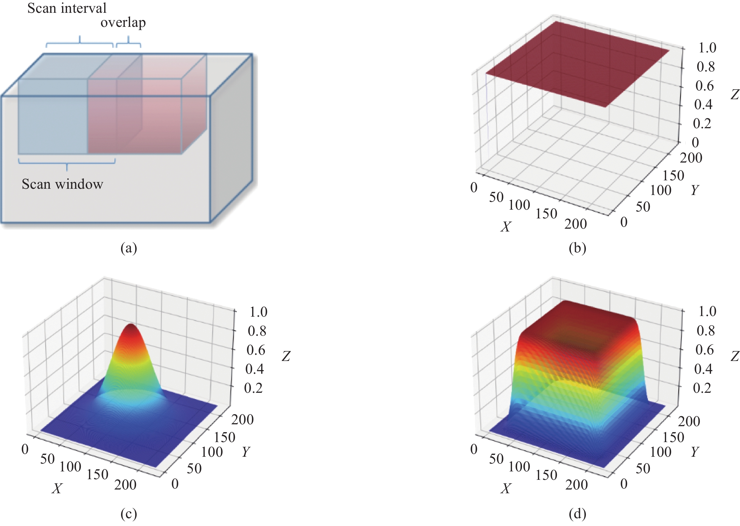
The inference is limited by GPU memory. A typical solution of that is using a scan window with overlapping[22], as shown in Fig.3(a). The whole volume inference requires several times of scan window inferences, and the calculation formula is given below:
Figure
3.
(a) Whole volume inference using scan window, (b) Filter kernel of average smoothing strategy, (c) Filter kernel of Gaussian smoothing strategy, (d) A new filter kernel and smoothing strategy designed to eliminate artifacts and speed up inference. All kernels of 2D cases are shown for convenience
Where n represents image dimension, sizei(n) and sizeinterval(n) are the size of the input volume and scan interval, respectively.
After scan window inferences, how to fuse the result of scan windows especially the overlapped region is a key problem. An intuitive average smoothing method simply averages activations in overlapping regions. However, severe border artifacts result in accuracy degradation. Gaussian smoothing strategy is improved by [22] to better aggregate the results of each scan window by smoothing activation maps with a Gaussian kernel, which eliminates border artifacts in a time-consuming fashion. Considering inference accuracy and time, we propose a novel smoothing kernel as shown in Fig.3(d) and defined in Eq.(11):
K=Rect(xs,ys,zs)∗Gσ(x,y,z),
(11)
where Gσ(⋅) is a Gaussian kernel, Rect(⋅) is a rectangular function. s controls the size of flat area shown in Fig.3(d), and σ controls the descend sharpness. When setting s=x, our method kernel is same with Gaussian smooth kernel. We empirically choose s as 3/4 the size of the scan window and σ as 1/32 the size of the scan window.
The new smoothing kernel functions as a weight map to fuse softmax activations. Unlike Gaussian smoothing, our smoothing kernel has a higher weight on center regions and descends sharply near the border, which allows larger scan intervals for faster inference.
3.
Experiments
3.1
Details
All training and inference methods were carried out on an NVIDIA Tesla V100 GPU. MR images are normalized and the cropped in training and inference, and the fixed crop size is 224×224×192. To avoid overfitting, we applied random zoom, random scale and random flip during the training. Adam optimizer was used, and the learning rate was set to 2×10⁻⁴ initially with polynomial decay.
3.2
Evaluation
10 cases were taken out as test set, and the test set includes 5 cases with knee OA and 5 healthy cases. The remaining 144 cases are applied for 4-fold cross-validation. To evaluate the accuracy of knee joint segmentation, the Dice similarity coefficient (DSC) was used and defined as Eq.(12), whereas TP, FN, FP means true positive, false negative, and false positive respectively.
DSC=2TPTP+FN+FP.
(12)
Hausdorff distance (HD) is another overlapping index used for evaluation, which measures the distance between the ground truth-x and the predicted segmentation-y. Eq.(13) defines Hausdorff distance, where sup represents the supremum, inf the infimum and d is the Euclidean distance.
HD=max{supx∈Xinfy∈Yd(x,y),supy∈Yinfx∈Xd(x,y)}.
(13)
3.3
Results
3.3.1
Comparison of Loss Function.
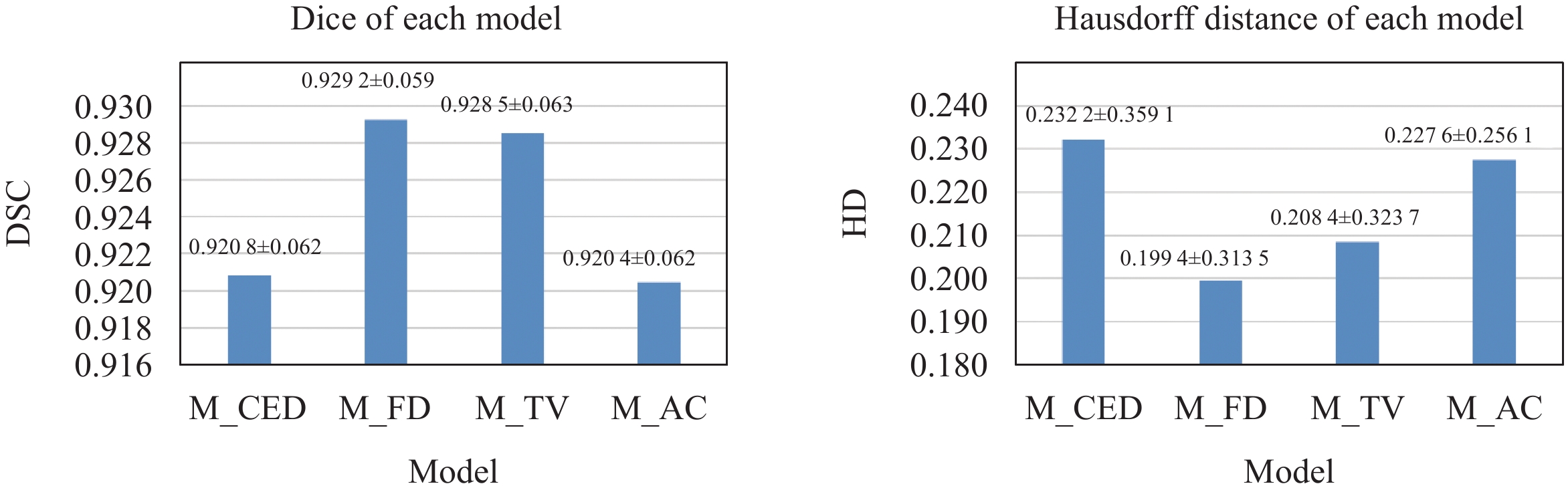
In this paper, a 4-fold cross-validation experiment was performed on 144 MR images. The test was performed on the other 10 MR images. Dataset is randomly sampled to ensure that each fold contains the same proportion of normal and OA scans. Models trained using different loss functions: CEDice, FocalDice, Tversky and AC, are named M_CED, M_FD, M_TV, and M_AC. Fig.4 shows the average DSC and HD of each model on test data. M_FD and M_TV significantly performed better.
In order to further compare the performance of diverse structures, statistics were made on the bone and soft tissue respectively, as shown in Fig.5. Models performed best on bones, and the accuracy is all above 97%. M_CED and M_AC had lower accuracy especially on cartilage. M_TV shows poor performance on posterior cruciate ligament and medial collateral ligament.
Figure
5.
Performance on different anatomical structures
Although there is a subtle difference in average accuracy of whole knee joint obtained from model with four different loss functions, when anatomical structures are compared separately, the gap between models will be noticeable. M_FD achieved better performance both on bone and soft tissue.
3.3.2
Analysis of Inference Strategies
Differences between the results of different inference strategies are shown in Table 1. The first row is the mean time for whole volume inference, the second row shows mean dice of test dataset, and prediction of one slice shows in the third row. It is obvious that there is wrong tibia prediction resulting from average smoothing inference, Gaussian smoothing and our smoothing method could improve prediction result. Our proposed inference strategy performs best in terms of time and accuracy.
Table
1.
Comparison of different inference strategies
There are two parameters in our inference smoothing kernel, and the effect of parameters is discussed below. We set scan window size as M, and compare the dice performance on soft tissue with different parameters. Table 2 shows the effect of each parameter. Smaller parameter σ makes a sharper kernel, it is similar with average smoothing kernel and resulting a worse dice performance. The parameter s controls the size of the flat area of the kernel function, a larger s means bigger valid overlapping regions and brings better dice performance.
The statistical results in the previous section have proved that M_FD is the most robust model, so the following analysis will be all performed on the M_FD. Fig.6 shows the average DSC and HD on 15 categories. The average DSC of the whole knee joint is about 92.92%. The DSC of four bones is the highest, all above 98%, followed by the patellar tendon and quadriceps tendon, with the DSC above 96%. The Dice of femur cartilage, tibia cartilage and medial meniscus are about 94%, patellar cartilage, lateral meniscus, ACL, PCL and MCL is between 87% ~ 90%, LCL is the lowest, about 76.34%. Also, the mean Hausdorff distance is 0.1994, and same with DSC, four bones get lowest HD, lateral meniscus get highest HD as 0.6934. LCL gets the lowest Dice Coefficient than other structures because lcl is the smallest structure and only accounts for 0.0245% of the whole volume. And compared with the state of art method-nnUNet[22], our model performs better on almost all anatomical structures.
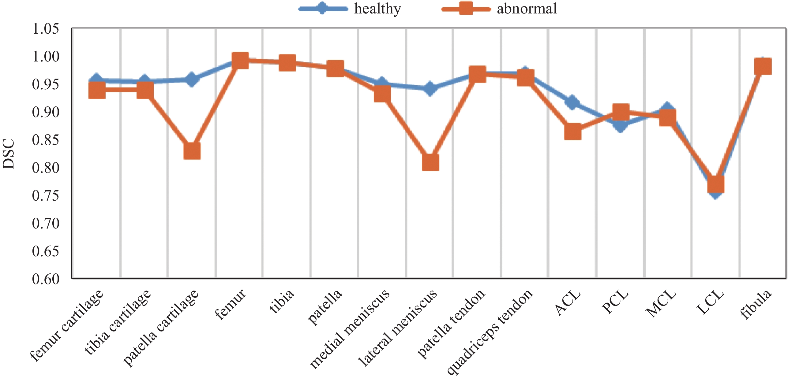
In order to compare the result on normal and abnormal scans more intuitively, Fig.7 shows the distribution of Dice more clearly. The accuracy of patella, lateral meniscus, and PCL are smaller than normal data, and the other 12 structures achieve almost the same segmentation accuracy as normal data, which proves the robustness of the model. For OA, lesion often appears in different locations. The varies proportion of different lesion results in different dice performance. Finally, segmentation results are shown in Fig.8.
Figure
7.
Performance comparison on normal and abnormal data
Figure
8.
Segmentation results. From left to right are: bone, quadriceps tendon and patellar tendon, collateral ligaments, cartilage, meniscus & cruciate ligaments, and whole segmented knee joint
In this study, we explored the feasibility of knee joint segmentation on fat-suppressed 3D isotropic medium-weight VISTA images, and implemented a network with an encoder-decoder structure to achieve whole knee 3D segmentation. In order to find a more robust segmentation model, we carried out experiments to evaluate the performance of multiple loss functions, and proved that the FocalDice is more robust to the segmentation of bone and soft tissues. A new smoothing strategy is further proposed to balance accuracy and inference time. The whole knee automatic segmentation in our experiment took about 40 seconds per subject, and the average DSC reached 92.92%. Future work will focus on improving the accuracy of lesion data segmentation, with the accumulation of labeled data with OA.
GUPTA S, HAWKER G A, LAPORTE A, et al. The economic burden of disabling hip and knee osteoarthritis (OA) from the perspective of individuals living with this condition[J]. Rheumatology (Oxford), 2005, 44(12): 1531−1537. DOI: 10.1093/rheumatology/kei049.
[2]
NIEMINEN M T, CASULA V, NEVALAINEN M T, et al. Osteoarthritis year in review 2018: Imaging[J]. Osteoarthritis anc Cartilage, 2019, 27(3): 401-411. DOI: 10.1016/j.joca.2018.12.009.
[3]
ECKSTEIN F, WIRTH W, CULVENOR A G. Osteoarthritis year in review 2020: Imaging[J]. Osteoarthritis and Cartilage, 2021, 29(2): 170−179. DOI: 10.1016/j.joca.2020.12.019.
[4]
ECKSTEIN F, CICUTTINI F, RAYNAULD J P, et al. Magnetic resonance imaging (MRI) of articular cartilage in knee osteoarthritis (OA): Morphological assessment[J]. Osteoarthritis and Cartilage, 2006, 14(A): 46−75. DOI: 10.1016/j.joca.2006.02.026.
[5]
BARR C, BAUER J, MALFAIR, D, et al. MR imaging of the ankle at 3 Tesla and 1.5 Tesla: Protocol optimization and application to cartilage, ligament and tendon pathology in cadaver specimens[J]. European Radiology, 2007, 17: 1518−1528. doi: 10.1007/s00330-006-0446-4
[6]
RAYNAULD J P, MARTEL-PELLETIER J, BERTHIAUME M J, et al. Long term evaluation of disease progression through the quantitative magnetic resonance imaging of symptomatic knee osteoarthritis patients: Correlation with clinical symptoms and radiographic changes[J]. Arthritis Research and Therapy, 2006, 8(1): R21.
[7]
HUNTER D J, MARCH L, SAMBROOK P N. The association of cartilage volume with knee pain[J]. Osteoarthritis and Cartilage, 2003, 11(10): 725−729. doi: 10.1016/S1063-4584(03)00160-2
[8]
ENGLUND M, GUERMAZI A, LOHMANDER L S. The meniscus in knee osteoarthritis[J]. Rheumatic Diseases Clinics of North America, 2009, 35(3): 579−590. doi: 10.1016/j.rdc.2009.08.004
[9]
LI R T, LORENZ S, XU Y, et al. Predictors of radiographic knee osteoarthritis after anterior cruciate ligament reconstruction[J]. The American Journal of Sports Medicine, 2011, 39(12): 2595−2603. doi: 10.1177/0363546511424720
[10]
SHARMA L, DUNLOP D, CAHUE S, et al. Quadriceps strength and osteoarthritis progression in malaligned and lax knees[J]. Annals of Internal Medicine, 2003, 138(8): 613−619. doi: 10.7326/0003-4819-138-8-200304150-00006
[11]
NORMAN B, PEDOIA V, MAJUMDAR S. Use of 2D U-net convolutional neural networks for automated cartilage and meniscus segmentation of knee MR imaging data to determine relaxometry and morphometry[J]. Radiology, 2018, 288(1): 177−185. DOI: 10.1148/radiol.2018172322.
[12]
PRASOON A, PETERSEN K, IGEL C, et al. Deep feature learning for knee cartilage segmentation using a triplanar convolutional neural network[C]//Medical Image Computing and Computer-Assisted Intervention: MICCAI International Conference on Medical Image Computing and Computer-Assisted Intervention, 2013, 16: 246-253.
[13]
GAJ S, YANG M, NAKAMURA K, et al. Automated cartilage and meniscus segmentation of knee MRI with conditional generative adversarial networks[J]. Magnetic Resonance in Medicine, 2020, 84(1): 437−449. doi: 10.1002/mrm.28111
[14]
ZHOU Z, ZHAO G, KIJOWSKI R, et al. Deep convolutional neural network for segmentation of knee joint anatomy[J]. Magnetic Resonance in Medicine, 2018, 80(6): 2759−2770. doi: 10.1002/mrm.27229
[15]
MYRONENKO A. 3D MRI brain tumor segmentation using autoencoder regularization[J]. Springer International Publishing, 2019.
[16]
WU Y X, HE K M. Group normalization[J]. International Journal of Computer Vision, 2020, 128: 742−755. doi: 10.1007/s11263-019-01198-w
[17]
TANG P, ZU C, HONG M, et al. DA-DSUnet: Dual attention-based dense SU-net for automatic head-and-neck tumor segmentation in MRI images[J]. Neurocomputing, 2021, 435: 103−113. doi: 10.1016/j.neucom.2020.12.085
[18]
ZHU W, HUANG Y, ZENG, L, et al. AnatomyNet: Deep learning for fast and fully automated whole‐volume segmentation of head and neck anatomy[J]. Medical Physics, 2018, 46(4): 576−589.
[19]
SALEH S S, ERDOGMUS D, GHOLIPOUR A. Tversky loss function for image segmentation using 3 D fully convolutional deep networks[J]. Machine Learning in Medical Imaging, 2017: 379−387.
[20]
CHEN X. WILLIAMS B M, VALLABHANENI S R, et al. Learning active contour models for medical image segmentation[C]//2019 Conference on Computer Vision and Pattern Recognition (CVPR), 2019: 11624-11632.
[21]
LIN T, GOYAL P, GIRSHICK R, et al. Focal loss for dense object detection[C]//2017 IEEE International Conference on Computer Vision (ICCV), 2017: 2999-3007.
[22]
ISENSEE F, JAEGER P F, KOHL S A, et al. Automated design of deep learning methods for biomedical image segmentation[J]. arXiv: 1904.08128, 2019.

 DownLoad: